Chinese Language Processing

This is part of CUPIDE (http://cupide.cse.cuhk.edu.hk).

Segmentation by maximal matching

There are quite a number of ways for Chinese segmentation. The simplest way of doing is maximal matching. Actually a lot of off-the-shelf Chinese segmentation library is based on this technique, examples include a number of PHP and Perl libraries and the very popular libtabe which used in the xcin for Chinese input in Linux.

The problem of maximal matching is that there are often ambiguities. Chen and Liu (1992) proposed a set of disambiguation rules for maximal matching. The first rule says that, the most plausible segmentation is the three word sequence with the maximal length, for example,

ABCDEFGH...

is a string where the dictionary contains:

A AB ABC B C BC CDEF GH DE F GH

It is an ambiguity in deciding how to segment the string headed with A. If we consider all the possible segmentation for the first three words, they are

A B C
A B CDEF
AB CDEF GH
AB C DE
ABC DE F

Then, the longest chunk is AB CDEF GH and we pick AB as the first word in the segmentation. The process continues in a recursive manners.

However, if the dictionary contains:

A AB ABC B C BC CDEF GH DE FGH

then we have two longest chunks:

AB CDEF GH
ABC DE FGH

The second rule of Chen and Liu proposes to pick the one with smallest SD in the word length. The first one has word lengths of 2, 4, 2 while the second one is 3, 2, 3. So it picks the second one. This rule is based on the heuristic that word length are usually evenly distributed.

Actually, there are four more rules in case the last two rules:

Pick the chunk with fewer bound morphemes (i.e. fewer characters)
Pick the chunk with fewer characters in determinative-measure compounds (pronouns, this, that etc are determinative, this rule means to pick the one with fewest word in phases begin with determinative)
Pick the chunk with the high frequently occurred monosyllabic words (i.e. in case ambiguity occurs by the choose of monosyllabic words, compare the frequency, in 的確實, 的 is more frequent than 實, so the correct segmentation is 的-確實)
Pick the chunk with the highest probability value (i.e. the sequence with greatest probability, in the sense of word Markov model, or the sum of word probability is highest, when one regards the words are discrete)

Tsai implemented Chen and Liu’s algorithm in his MMSEG. However, only the first two rules are implemented because the word frequency are not included in his lexicon.

Add-one smoothing

Also known as Laplace’s Law, is to give every entry of the language model (i.e. corpus data) a base count of one and then add the counted frequency from training data. The data is then normalized to give the probability. In other words, the probability \(p\) of word \(w\), with \(c\) counted occurrences in the training data of size \(N\), is given by \(p=(c+1)/(N+V)\), where \(V\) is the total number of distinct words in the model. Hence every unknown word has probability of \(1/(N+V)\).

Add-one smoothing does not provide good result because of the sparse nature of the language model, i.e. \(V\) is very large. Hence the probability is distorted a lot for frequent terms because of the normalization.

Good-Turing discounting

Use the items that we saw once to estimate the probability of unseen terms. The items that occurred once is called a singleton or hapax legomenon.

We define the frequency of frequency \(k\) to be \(N_k = \displaystyle\sum_{w:\textrm{count}(w)=k} 1\), i.e. the number of entries with frequency \(k\). Then the adjusted count is defined by \(c^\ast = (c+1)\frac{N_{c+1}}{N_c}\). It turns out that the probability of a term that occurred \(c\) times in the training data is \(p=c^{\ast}/N\).

The high frequency counts are assumed to be reliable, hence adjusted count is not applied to the high frequency terms. Katz (1987) suggested that for \(c\) greater than \(k=5\), we use \(c^{\ast}=c\). Katz (1987) also suggested to use a finer adjustment for \(c^{\ast}\) when \(1\le c\le k\):

\[c^{\ast}= \frac{(c+1)\frac{N_{c+1}}{N_c}-c\frac{(k+1)N_{k+1}}{N_1}}{1-\frac{(k+1)N_{k+1}}{N_1}}\]

Good-Turing discounting will give probability of zero occurrence terms similar to that of a singleton.

Katz Backoff

Backoff is to make use of lower-order \(n\)-gram to compute the probability of higher-order \(n\)-gram. For example, we use the information of unigram to compute the probability of bigram.

Assume we have a \(n\)-gram of the form \(w_{n-k}...w_{n-2}w_{n-1}w_{n}\) which is denoted by \(w_{n-k}^{n}\) and its probability is defined as \(P(w_{n-k}^{n})\). Then the probability of a word given the previous \((N-1)\)-gram is:

\[P_K(w_n|w_{n-N+1}^{n-1})=\begin{cases} P^{\ast}(w_n|w_{n-N+1}^{n-1}) & \textrm{if }C(w_{n-N+1}^{n-1})>0 \\ \alpha(w_{n-N+1}^{n-1})P_K(w_n|w_{n-N+2}^{n-1}) & \textrm{otherwise} \end{cases}\]

where the discounted probability \(P^{\ast}\) is computed based on the discounted count \(c^{\ast}\)

\[P^\ast(w_n|w_{n-N+1}^{n-1})=\frac{c^\ast(w_{n-N+1}^{n})}{c(w_{n-N+1}^{n-1})}\]

and \(\alpha\) is the normalizing factor, which is

\[\alpha(w_{n-N+1}^{n-1})= \frac{1-\displaystyle\sum_{w_n:C(w_{n-N+1}^n)>0}P^\ast(w_n|w_{n-N+1}^{n-1})} {1-\displaystyle\sum_{w_n:C(w_{n-N+1}^n)>0}P^\ast(w_n|w_{n-N+2}^{n-1})}\]

Interpolation

Computing the probability of any \(n\)-gram by the weighted sum of the measured probability of associated \(n\)-gram, \((n-1)\)-gram, \((n-2)\)-gram, etc.

Part-of-Speech

POS tagging helps language processing. In English, following part-of-speech categorization is commonly used:

Closed classes: Relatively fixed set
- prepositions: on, under, over, near, by, at, from, to, with
- determiners: a, an, the
- pronouns: she, who, I, others
- conjunctions: and, but, or, as, if, when
- auxiliary verbs: can, may, should, are
- particles: up, down, on, off, in, out, at, by
- numerals: one, two, three, first, second, third
Open classes
- nouns
  - proper nouns: IBM, Google, England
  - common nouns
    - count nouns: Countable ones, with singular and plural form, e.g. goats, cats
    - mass nouns: e.g. snow, communism
- verbs
- adjectives
- adverbs
  - directional adverb/locative adverb: here, there
  - degree adverb: extremely, likely
  - manner adverb: slowly, delicately
  - temporal adverb: today, yesterday

POS tagging in English text is commonly done by HMM.

Resources

Prof Chih-Hao Tsai’s page has a lot of word-frequency stuff on Chinese: http://technology.chtsai.org/
- his maximal matching segmentation with disambiguation rules: http://technology.chtsai.org/mmseg/
Google’s stop word list on English
A long list of English stopwords

@INPROCEEDINGS{cl92,
    title = {Word Identification for Mandarin Chinese Sentences},
    author = {Keh-Jiann Chen and Shing-Huan Liu},
    year = 1992,
    month = Aug,
    booktitle = {15th International Conference on Computational Linguistics},
    file = {https://drive.google.com/open?id=0B6DoI_vm0OLfbUUtaTlYUzB4X0k),
}

Segmentation by maximum entropy approach

In Low et al (2005), it proposed the use of maximum entropy to perform segmentation. The idea is to identify the beginning and ending of a “word” by considering the contextual clues. It relies on a large corpus which tells what is a word in Chinese text. It tags the beginning character of a word by “L” and the ending character by “R”, while all the middle characters are tagged with “M”, if any. Then, a word can be identified if we can also do the similar thing on the inputted text. See (Xue and Shen, 2003).

It is a learning algorithm, such that the corpus teaches how the words shall be tagged. The corpus not only tells about the correct tagging, but also the other “features” that assists the tagging. All these kind of information is then feed into a maximum entropy model which uses the EM algorithm to deduce the optimal parameters. This is called the training process. The trained model is then used for the subsequent segmentation.

However, there are four problems with this approach: (1) The features extracted may affect (lead or mislead) the model; (2) The corpus has to be very large and hundred percent correct to make a perfect model; (3) Training takes a long time; (4) There could be strange results: it is not necessarily know L→M→R is a fixed sequence and R→M→L is not allowed, because the tagging is character by character based on context clues only.

Lau and King (2005) proposes a two-stage training to avoid a very large corpus: Train the model with just half of the corpus and use this trained model to tag the second half of the corpus. Mistakes are expected but we compare the mistaken tagging with the correct one and train the model again with the tagged result as additional features. The double-trained model can produce results more accurately.

I think it is OK for problems (1)-(3) exist. However, problem (4) means the system is not tagging correctly (in the sense that it is illogical to have such tagging result). Any solution for this? May be we should build a Markov chain to tell that R→M is impossible.

@INPROCEEDINGS{lng05,
    title = {A Maximum Entropy Approach to Chinese Word Segmentation},
    author = {Jin Kiat Low and Hwee Tou Ng and Wenyuan Guo},
    year = 2005,
    booktitle = {Fourth SIGHAN Workshop on Chinese Language Processing},
    url = {http://www.comp.nus.edu.sg/~nght/pubs/sighan05.pdf}
}
@INPROCEEDINGS{xs03,
    title = {Chinese Word Segmentation as LMR Tagging},
    author = {Nianwen Xue and Libin Shen},
    booktitle = {Second SIGHAN Workshop on Chinese Language Processing},
    year = 2003,
    url = {http://acl.ldc.upenn.edu/acl2003/sighan/pdf/XueShen.pdf}
}
@INPROCEEDINGS{lk05,
    title = {Two-Phase LMR-RC Tagging for Chinese Word Segmentation},
    author = {Tak Pang Lau and Irwin King},
    year = 2005,
    booktitle = {Fourth SIGHAN Workshop on Chinese Language Processing},
    url = {http://acl.ldc.upenn.edu/I/I05/I05-3031.pdf}
}

Segmentation by n-gram

Google’s research blog has an entry in last summer mentioning they uses \(n\)-gram to do text processing

Actually, \(n\)-gram can help doing Chinese segmentation, for example, an algorithm is described in a blog entry

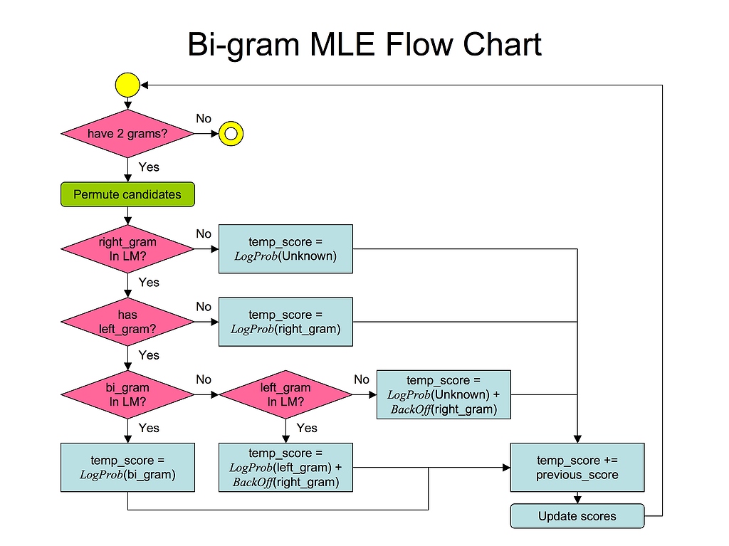
The above is the flow chart about the algorithm. The segmentation is done as a dynamic programming problem:

INPUT: string[]    // input string to segment
INPUT: model[]     // n-gram model

ARRAY: score[]     // max score for running to a particular position
ARRAY: lastHop[]   // last hop of a particular position for which attains that max score

pos = 0
// Scan the whole input string
for pos=0 to length(string[])
    for i=0 to pos
        leftPiece = substring(string, from pos-i to pos)
        if (not found model[leftPiece])
            // set the max score of going to this position
            tempScore = score[pos-i-1] + probability(unknown piece)
            if (tempScore > score[pos])
                score[pos] = tempScore
                lastHop[pos] = pos-i
            end if
            next
        end if
        for j=pos+1 to length(string[])
            rightPiece = substring(string, from pos to j)
            // if we don't have rightPiece, update scores according to leftPiece
            if (rightPiece = NULL)
                tempScore = score[pos-i-1] + probability(leftPiece)
                if (tempScore > score[pos])
                    score[pos] = tempScore
                    lastHop[pos] = pos-i
                end if
                next
            end if
            // if we have rightPiece, check if we can combine them to form a bigger n-gram
            if (found model[leftPiece + rightPiece])
                tempScore = score[pos-i-1] + probability(leftPiece + rightPiece)
            // if we cannot combine them, check if rightPiece is known
            else if (found model[rightPiece])
                tempScore = score[pos-i-1] + probability(leftPiece) + probability(rightPiece) + smoothing()
            // if neither, use alternative way to combine
            else
                tempScore = score[pos-i-1] + probability(leftPiece) + probability(unknown piece) + smoothing()
            end if
            // update the scoring
            if (tempScore > score[j])
                score[j] = tempScore
                lastHop[j] = pos-i
            end if
        end for
    end for
end for

pos = length(string[])
bestTrail[] = empty
while pos>0
    bestTrial[] = prepend lastHop[pos] to bestTrial[]
    pos = lastHop[pos]
end while

output bestTrial[]

The above code employs a smoothing algorithm for estimating the probability of unknown \(n\)-gram. The most popular one is the Katz’s algorithm.

The author suggested that the probability used in the above code should be log-probability, hence the total score is actually the log-probability of a sentence.

My comment: The \(n\)-gram model is actually a union of the unigram, bigram, trigram, quadrigram, pentagram, etc. Hence the probability should not be comparable between. I wonder whether the above algorithm favors single-character segmentation, because of the smaller cardinal size of unigram than other \(n\)-gram.

Put it simple, assume two characters \(C_1\) and \(C_2\) are both very common in the unigram. And \(C_1C_2\) is a valid phrase and therefore, \(C_1C_2\) is also common in the bigram. Can one tell if the probability of \(C_1\) in unigram is less than that of \(C_1C_2\) in bigram?

Smoothing in n-gram

Smoothing \(n\)-gram means to fill-in the probabilities of unseen entries besides those evaluated from the training data.

References:

@ARTICLE{k87,
    author = {Katz, S. M.},
    year = 1987,
    title = {Estimation of probabilities from sparse data for the language model component of a speech recogniser},
    journal = {IEEE Transactions on Acoustics, Speech, and Signal Processing},
    volume = 35,
    number = 3,
    pages = {400--401}
}
@INCOLLECTION{jm06,
    author = {Daniel Jurafsky and James H. Martin},
    title = {n-grams},
    chapter = 4,
    booktitle = {Speech and Language Processing: An introduction to speech recognition, 
computational linguistics and natural language processing},
    year = 2006
}