Beta distribution

If we have a coin, how do we know it is fair? Indeed we never know for sure. But if we flip it enough time, we may learn enough about the coin to tell with certain confidence that the coin is fair or not. That is how beta distribution comes to play.

Let us model the coin to have two sides, head and tail, and when we flip it, it will land on either side. We are interested in the probability \(p\) of, say, it lands on head. This implicitly defines the probability of it lands on tail to be \(1-p\). If we have no knowledge about the coin at all, we either:

1. assume any \(p\in[0,1]\) is equally possible; or
2. saw the coin has head but not even sure the flip side is tail

Or anything even weirder. Beta distribution, has the density function

As the prior, if \(\alpha=\beta=1\), we have a horizontal curve that correspond to the first case. If \(\alpha=\beta=0\), the gamma functions are undefined and may be this reflects the case of absolutely no knowledge about the coin. What beta distribution models is the probability of the value of \(p\) (i.e., probability of a probability): if we carry out a Bernoulli trial with the coin, and it turns out to have \(n\) heads and \(N-n\) tails, then the probability of the actual value of \(p\) follows the density of beta distribution with \(\alpha=n+\alpha_0\) and \(\beta=N-n+\beta_0\), which \(\alpha_0\) and \(\beta_0\) are the prior.

These are the standard usage of beta distribution, but the interesting part is how many Bernoulli trials needed to give us confidence to the value of \(p\). Of course, one way to measure this is the variance of the distribution, namely,

but we can also use the Shannon entropy

which \(B(\alpha,\beta)\) is the beta function and \(\chi(x)\) is the digamma function. Simulating a Bernoulli trial with different actual value of \(p\), derive the corresponding beta distribution function, and plotting the entropy against trial count gives the following:

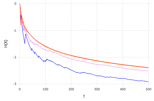
Curves on plot in red, orange, violet, and blue are respectively using \(p\) of 0.5, 0.6, 0.75, and 0.9. We see the following:

1. Shannon entropy is negative as expected, because the distribution is continuous. This does not tell us how many bits of information are provided (which is provided by differential entropy), but rather, a relative scale of information
2. As the trial goes on, the entropy is decreasing. Theoretically, once we know the exact value of \(p\) from experiment, we reach the entropy level of zero
3. Law of diminishing return observed: rapid drop of entropy at beginning and slowed down afterwards
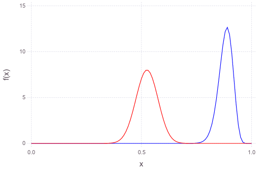
4. \(p=0.9\) has lower entropy level than \(p=0.5\) but that barely means \(p=0.9\) is much less interesting, and thus making the pdf of beta distribution narrower (higher kurtosis), as shown in the following:

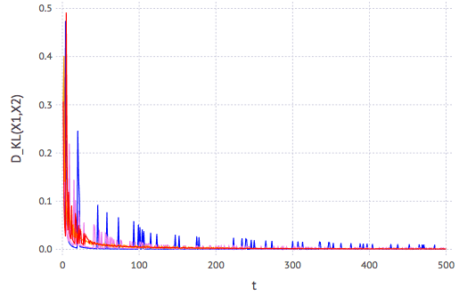
It seems that, no matter what \(p\) actually be, we need only around 30 Bernoulli trials to get a fairly good (and cost-effective) estimate. This can be easier seen using K-L divergence metric of the distributions between successive trial:

Julia code to generate the previous plots

using Gadfly

# distribution, entropy, and divergence of beta distribution
betapdf(x,a,b) = x^(a-1)*(1-x)^(b-1)*gamma(a+b)/gamma(a)gamma(b)
H(a,b) = log(beta(a,b))-(a-1)digamma(a)-(b-1)digamma(b)+(a+b-2)digamma(a+b)
D(a1,b1,a2,b2) = log(beta(a2,b2)/beta(a1,b1)) + (a1-a2)digamma(a1) + (b1-b2)digamma(b1) + (a2-a1+b2-b1)digamma(a1+b1)

function trial(p, a0, b0, N)
    # initial beta param a0, b0, flip coin with prob p, update (ai,bi), up to (aN,bN)
    a, b, x = zeros(N+1), zeros(N+1), rand(N)
    a[1] = a0
    b[1] = b0
    for i in 1:N
        if x[i] > p
            a[i+1] = a[i]
            b[i+1] = b[i] + 1
        else
            a[i+1] = a[i] + 1
            b[i+1] = b[i]
        end
    end
    return [a b] # Nx2 matrix
end
N = 500
param1 = trial(0.5, 1, 1, N)
param2 = trial(0.6, 1, 1, N)
param3 = trial(0.75, 1, 1, N)
param4 = trial(0.9, 1, 1, N)

# Plot H(X) against t
x = 1:N
y1 = [H(param1[i,1], param1[i,2]) for i=x]
y2 = [H(param2[i,1], param2[i,2]) for i=x]
y3 = [H(param3[i,1], param3[i,2]) for i=x]
y4 = [H(param4[i,1], param4[i,2]) for i=x]
plot(layer(x=x, y=y1, Geom.line, Theme(default_color=colorant"red")),
     layer(x=x, y=y2, Geom.line, Theme(default_color=colorant"orange")),
     layer(x=x, y=y3, Geom.line, Theme(default_color=colorant"violet")),
     layer(x=x, y=y4, Geom.line, Theme(default_color=colorant"blue")),
     Guide.XLabel("t"), Guide.YLabel("H(X)"))

# Plot K-L divergence against t
y1 = [D(param1[i,1], param1[i,2], param1[i+1,1], param1[i+1,2]) for i=x]
y2 = [D(param2[i,1], param2[i,2], param2[i+1,1], param2[i+1,2]) for i=x]
y3 = [D(param3[i,1], param3[i,2], param3[i+1,1], param3[i+1,2]) for i=x]
y4 = [D(param4[i,1], param4[i,2], param4[i+1,1], param4[i+1,2]) for i=x]
plot(layer(x=x, y=y1, Geom.line, Theme(default_color=colorant"red")),
     layer(x=x, y=y2, Geom.line, Theme(default_color=colorant"orange")),
     layer(x=x, y=y3, Geom.line, Theme(default_color=colorant"violet")),
     layer(x=x, y=y4, Geom.line, Theme(default_color=colorant"blue")),
     Guide.XLabel("t"), Guide.YLabel("D_KL(X1,X2)"))

Extension: Fair dice

Outcome of a coin is binary, but a dice is 6-ary. Beta distribution is a scalar function and we need a vector function to model the outcome of a dice. The generalisation of beta distribution to multivariate form is Dirichlet distribution, whose density function is

which defined for \(\sum_{i=1}^k x_i=1,\ x_i\in(0,1)\) and \(\alpha_i>0\). A sequence of trial of dice roll updates \(\vec{\alpha}\) as above. The Dirichlet distribution gives the probability estimation of each face of dice. The distribution can be computed as follows, using beta distribution recursively:

As another application, we can model the multilevel review (e.g., one-star to five-star as in Amazon) as Dirichlet distribution and use its entropy to rate the trustworthiness of such review.