Multivariate normal distribution has the following p.d.f.:
\[f(\vec{x}) = \frac{1}{\sqrt{(2\pi)^n|\mathbf{\Sigma}|}} \exp(-\frac{1}{2}(\vec{x}-\vec{\mu})^T\mathbf{\Sigma}^{-1}(\vec{x}-\vec{\mu}))\]and for a bivariate in specific, it is:
\[f(x_1,x_2) = \frac{1}{2\pi\sqrt{\sigma_1^2\sigma_2^2-\sigma_{12}^2}} \exp\left(-\frac{ \sigma_2^2(x_1-\mu_1)^2 - 2\sigma_{12}(x_1-\mu_1)(x_2-\mu_2) + \sigma_1^2(x_2-\mu_2)^2 }{ 2(\sigma_1^2\sigma_2^2-\sigma_{12}^2) } \right)\]where the covariance \(\sigma_{12}^2 = \rho\sigma_1\sigma_2\). See also the note on multivariate Gaussian distribution.
The multivariate normal random variable can be considered as a combination of the mean vector and zero-mean multivariate random variable. Assume \(\mathbf{y}\) to be a \(n\)-vector of iid standard normal random variables, i.e., \(\bar{\mathbf{y}}=\mathbf{0}\) and \(E[\mathbf{yy}^T]=\mathbf{I}\). Let there be a matrix of constants \(\mathbf{S}\) of size \(m\times n\), and a \(m\)-vector of constants (the mean) \(\mathbf{m}\), and define
\[\mathbf{x} = \mathbf{Sy} + \mathbf{m}\]Then \(\mathbf{x}\) is a multivariate normal random variable, which the covariance matrix is
\[\begin{align} \Sigma_{\mathbf{x}} &= E[(\mathbf{x}-\mathbf{m})(\mathbf{x}-\mathbf{m})^T] \\ &= E[(\mathbf{Sy})(\mathbf{Sy})^T] \\ &= E[\mathbf{Sy}\mathbf{y}^T\mathbf{S}^T] \\ &= \mathbf{S}E[\mathbf{yy}^T]\mathbf{S}^T \\ &= \mathbf{SS}^T \end{align}\]Finding \(\mathbf{S} = \Sigma_{\mathbf{x}}^{1/2}\) given covariance matrix \(\Sigma_{\mathbf{x}}\) is typically using Cholesky decomposition.
Taking again bivariate as an example. If the covariance matrix is
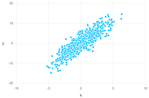
\[\Sigma_{\mathbf{x}} = \begin{bmatrix}3 & 2 \\ 2 & 5\end{bmatrix}\]In Julia, we can plot a set of samples of the distribution as follows (assumed zero-mean):
Sigma = [4 9; 9 25]
S = chol(Sigma) # upper triangular part, i.e. S' * S == Sigma
iidnorm = randn(2,1000)
mvnorm = S' * iidnorm
using Gadfly
plot(x=mvnorm[1,:], y=mvnorm[2,:], Geom.point)
Alternatively, such sampling can also be done using Monte Carlo method, such as the Gibbs sampling. The algorithm is Gibbs sampling is as follows:
- Assume some sensible value for the multivariate random variable \(x^{(0)} = (x_1^{(0)}, x_2^{(0)}, \cdots, x_n^{(0)})\) as initial value
- For \(k=0\) up to \(k=M+N\)
- For \(i=1\) up to \(i=n\), i.e. each component of the multivariate random variable
- Set \(x_i^{(k+1)}\) according to probability \(p(x_i\mid x_1^{(k+1)}, \cdots, x_{i-1}^{(k+1)}, x_{i+1}^{(k)}, \cdots, x_n^{(k)})\)
- For \(i=1\) up to \(i=n\), i.e. each component of the multivariate random variable
- Discard the first \(M\) samples of \(x^{(k)}\) above and use only the last \(N\) as terminal distribution
For the particular case of zero-mean bivariate normal random variables, the loop above means:
- For \(k=0\) up to \(k=M\)
- set \(x_1^{(k+1)} = \rho x_2^{(k)}\sigma_1/\sigma_2 + \sqrt{\sigma_1^2(1-\rho^2)} Z_1\) where \(Z_1 \sim N(0,1)\)
- set \(x_2^{(k+1)} = \rho x_1^{(k+1)}\sigma_2/\sigma_1 + \sqrt{\sigma_2^2(1-\rho^2)} Z_2\) where \(Z_2 \sim N(0,1)\)
The formula \(x_1^{(k+1)} = \rho x_2^{(k)} + \sqrt{\sigma_1^2(1-\rho^2)} Z_1\) comes from the following:
\[\begin{align} p(x_1 \mid x_2) &= \frac{p(x_1, x_2)}{p(x_2)} \\ &= \frac{ \frac{1}{2\pi\sigma_1\sigma_2\sqrt{1-\rho^2}} \exp\left( -\frac{x_1^2/\sigma_1^2 - 2\rho x_1x_2/(\sigma_1\sigma_2)+x_2^2/\sigma_2^2}{2(1-\rho^2)} \right) }{ \frac{1}{\sqrt{2\pi\sigma_2^2}} \exp\left(-\frac{x_2^2}{2\sigma^2}\right) } \\ &= \frac{1}{\sqrt{2\pi}\sigma_1\sqrt{1-\rho^2}} \exp\left( -\frac{(x_1/\sigma_1 - \rho x_2/\sigma_2)^2}{2(1-\rho^2)} \right) \\ &= \frac{1}{\sqrt{2\pi}\sigma_1\sqrt{1-\rho^2}} \exp\left( -\frac{(x_1 - \rho x_2\sigma_1/\sigma_2)^2}{2\sigma_1^2(1-\rho^2)} \right) \\ &= N(\rho x_2\sigma_1/\sigma_2, \sigma_1^2(1-\rho^2)) \end{align}\]And this is the corresponding code:
Sigma = [4 9; 9 25]
sigma1 = sqrt(Sigma[1,1])
sigma2 = sqrt(Sigma[2,2])
rho = Sigma[1,2]/(sigma1*sigma2)
states = []
push!(states, [0,0])
for i = 1:1500
Z1,Z2 = randn(2)
x1, x2 = last(states)
x1 = rho * x2 * sigma1 / sigma2 + sqrt(sigma1^2 * (1-rho^2)) * Z1
x2 = rho * x1 * sigma2 / sigma1 + sqrt(sigma2^2 * (1-rho^2)) * Z2
push!(states, [x1,x2])
end
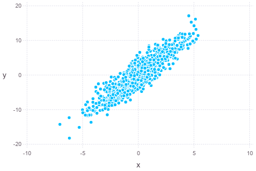
states = hcat(states...)
plot(x=states[1,501:end], y=states[2,501:end], Geom.point)