If you search “cantopop” in YouTube, you will find loads of music videos. Each of the video will bear a title. Below are some examples:
  HOCC何韻詩《代你白頭》MV
  林二汶 Eman Lam - 愛情是一種法國甜品
  [JOY RICH] [舊歌] 張國榮 - 有心人(電影金枝玉葉2主題曲)
  張學友 _ 李香蘭 (高清音)
  衛蘭 Janice Vidal - 伯利恆的主角 The Star Of Bethlehem (Official Music Video)
  張敬軒 Hins Cheung - 酷愛 (Hins Live in Passion 2014)
Can we figure out the name of the artist and the name of the song from the title?
This problem is closely similar to the problem of segmentation in the first sight. The problem of Chinese segmentation is to identify phases from a string of characters, which then we can look up a dictionary or otherwise, identify each phases part of speech. One of the way to do segmentation is to train a hidden Markov model or using LSTM. However, I don’t think this approach is applicable here – for a segmentation problem usually work on a fairly long sentence and train with a massive data, which the phases are supposed to be repeated fairly often. The problem here does not fit. Firstly, quite often we know how to segment the title: There are punctuations to group ideograph characters. Secondly, tagging the segmented phases by dictionary means we have a full dictionary of all artist names and songs, which the problem would be trivial if we have one and it can’t cope with new entries.
Of course, we can assume that the name of the song vs the name of the artist would bias to a different subset of characters. But we can also base on some contextual hints. For example, we can expect the phase inside 《..》 is the name of the song and the short phase closer to the beginning of the title is more likely than not the name of the artist. Instead of figuring out the rules to do this, we can learn through data and build an engine. Here I use scikit-learn.
Preparation of data
We collected a few hundred of cantopop titles from YouTube. Then we segmentize them and convert the tokens into features as follows:
def condense(tagged: Iterable[Tuple[str, str]]) -> Iterable[Tuple[str, str]]:
    "Aggregate pairs of the same tag"
    tag, string = None, ''
    for t,s in tagged:
        if tag == t:
            string += s
        elif tag is None:
            tag, string = t, s
        else:
            yield (tag, string)
            tag, string = t, s
    if tag is not None:
        yield (tag, string)

def latincondense(tagged: Iterable[Tuple[str, str]]) -> Iterable[Tuple[str,str]]:
    "Aggregate Latin words (Lu then Ll) into one tuple and mangle the space (Zs) type"
    dash = ['-', '_', '\u2500', '\uff0d', ]
    tag, string = None, ''
    for t,s in tagged:
        if (tag, t) == ('Lu','Ll'):
            tag, string = 'Lul', string+s
        elif tag is None:
            tag, string = t, s
        else:
            if tag == 'Zs':
                yield (tag, ' ')
            elif tag in ['Pc','Pd'] and string in dash:
                yield ('Pd', '-')
            else:
                yield (tag, string)
            tag, string = t, s
    if tag is not None:
        yield (tag, string)

def strcondense(tagged: Iterable[Tuple[str,str]]) -> List[Tuple[str,str]]:
    "Condense latin string phases into one tuple, needs look ahead"
    strtype = ['Lu', 'Ll', 'Lul', 'Lstr']
    tagged = list(tagged)
    i = 1
    # Condense string into Lstr tag
    while i < len(tagged):
        # combine if possible, otherwise proceed to next
        if tagged[i][0] in strtype and tagged[i-1][0] in strtype:
            tagged[i-1:i+1] = [('Lstr', tagged[i-1][1]+tagged[i][1])]
        elif i>=2 and tagged[i][0] in strtype and tagged[i-1][0] == 'Zs' and tagged[i-2][0] in strtype:
            tagged[i-2:i+1] = [('Lstr', tagged[i-2][1]+' '+tagged[i][1])]
            i = i-1
        else:
            i += 1
    return tagged

def features(title: str) -> List[dict]:
    '''Convert a title string into features'''
    stopword = ['MV', 'Music Video', '歌詞', '高清', 'HD', 'Lyric Video', '版']
    quotes = ['()', '[]', '《》', '【】', '()', "“”", "''", '""',  ] # Ps and Pe, Pi and Pf, also Po
    # condense string with tags
    tagstr = strcondense(latincondense(condense( [(unicodedata.category(c), c) for c in title] )))
    # add other features: within quote (for diff quotes), is before dash, is
    # after dash, strlen count, tok count, Lo tok count, str is in name set, str
    # is in stopword set
    qpos = {}
    strlen = 0
    Lo_cnt = 0
    vector = []
    # position offset features, forward and backward
    for i, (t, s) in enumerate(tagstr):
        vector.append(dict(
            str=s, tag=t, ftok=i+1, flen=strlen, slen=len(s),
            stopword=any(w in s for w in stopword)
        ))
        if t == 'Lo':
            Lo_cnt += 1
            vector[-1]['fzhtok'] = Lo_cnt
        strlen += len(s)
    for tok in vector:
        tok.update({
            'titlen': strlen,
            'btok': len(vector) + 1 - tok['ftok'],
            'blen': strlen - len(tok['str']) - tok['flen'],
        })
        if 'fzhtok' in tok:
            tok['bzhtok'] = Lo_cnt + 1 - tok['fzhtok']
    # bracket features
    for key in quotes + ['-']:
        qpos[key] = []
    for tok in vector:
        if tok['tag'] == 'Pd':
            qpos['-'].append(tok['ftok'])
        else:
            for quote in quotes:
                if tok['str'] in quote:
                    qpos[quote].append(tok['ftok'])
                    break
    for tok in vector:
        try:
            tok['dashbefore'] = tok['ftok'] > min(qpos['-'])
            tok['dashafter'] = tok['ftok'] < max(qpos['-'])
        except ValueError:
            pass
        for quote in quotes:
            if not qpos[quote]:
                continue
            inquote = [1 for i,j in zip(qpos[quote][::2], qpos[quote][1::2]) if i < tok['ftok'] < j]
            tok[quote] = bool(inquote)
    return vector
The above code is to segmentize the title string based on the unicode character category, for we expects CJK ideograph and Latin alphabets mixed with punctuations and spaces. We do not try to further segmentize a string of CJK ideographs into phrases but treat it as a whole. We also normalize different forms of dash into one and identify stopwords based on substring matching. The features of each segmentized tokens are assigned based on length (titlen and slen), the position (ftok, btok, flen, blen, fzhtok, bzhtok, for counting forward and backward, based on characters and tokens), and neighbours (dashbefore, dashafter, (), [], 《》, 【】, (), “”, '', "", mostly to identify whether the token is surrounded by a pair of different type of brackets/quotes).
With these features created from the tokens, we manually label which one corresponds to the name of artist, name of the song, and everything else. Now we have a problem of multiclass classification: Only not sure which algorithm is the best to train and apply.
Comparing different classifiers
There is a beautiful chart at scikit’s auto examples that compares different classifiers with different nature of data. Unfortunately this is only for 2D (two input features) but we have a higher dimension. We will forget about the graphics but focus only on the classification accuracy for now. Here is what we do for classification test:
#!/usr/bin/env python
# coding: utf-8

#
# Classifier demo
#
# Some code are derived from
# https://scikit-learn.org/stable/auto_examples/classification/plot_classifier_comparison.html

import pickle

import pandas as pd
import numpy as np
# scikit-learn utility functions
from sklearn.model_selection import train_test_split
from sklearn.metrics import classification_report
# different classifiers
from sklearn.linear_model import LogisticRegression
from sklearn.neural_network import MLPClassifier
from sklearn.neighbors import KNeighborsClassifier
from sklearn.svm import SVC
from sklearn.gaussian_process import GaussianProcessClassifier
from sklearn.gaussian_process.kernels import RBF
from sklearn.tree import DecisionTreeClassifier
from sklearn.ensemble import RandomForestClassifier, AdaBoostClassifier
from sklearn.naive_bayes import GaussianNB
from sklearn.discriminant_analysis import QuadraticDiscriminantAnalysis


#
# Define classifiers
#

classifiers = [
     ("Logistic Regression", LogisticRegression(solver='newton-cg', max_iter=1000, C=1, multi_class='ovr'))
    ,("Nearest Neighbors", KNeighborsClassifier(3))
    ,("Linear SVM", SVC(kernel="linear", C=0.025))
    ,("RBF SVM", SVC(gamma=2, C=1))
    ,("Decision Tree", DecisionTreeClassifier(max_depth=5))
    ,("Random Forest", RandomForestClassifier(max_depth=5, n_estimators=10, max_features=1))
    ,("Neural Net", MLPClassifier(alpha=0.01, max_iter=1000))
    ,("AdaBoost", AdaBoostClassifier())
    ,("Naive Bayes", GaussianNB())
    ,("Gaussian Process", GaussianProcessClassifier(1.0 * RBF(1.0)))
    ,("QDA", QuadraticDiscriminantAnalysis())
]


#
# Prepare for plotting and classification
# df is the input data of feature vectors and labels
# incol is all feature columns
# 'label' is the classification label, i.e., the expected result
#

X = df[incol]
y = df['label']

#
# Train, evaluate, and plot
#

# preprocess dataset, split into training and test part
X_train, X_test, y_train, y_test = train_test_split(X, y, test_size=.4, random_state=1841)

# iterate over classifiers and plot each of them
for name, clf in classifiers:
    # train and print report
    clf.fit(X_train, y_train)
    score = clf.score(X_test, y_test)
    print("----\n{} (score={:.5f}):".format(name, score))
    print(classification_report(y_test, clf.predict(X_test), digits=5))
and this is the result:
Logistic Regression (score=0.93935):
              precision    recall  f1-score   support

           a    0.78919   0.76842   0.77867       190
           t    0.82099   0.73889   0.77778       180
           x    0.96966   0.98427   0.97691      1526

    accuracy                        0.93935      1896
   macro avg    0.85994   0.83053   0.84445      1896
weighted avg    0.93746   0.93935   0.93814      1896
----
Nearest Neighbors (score=0.91139):
              precision    recall  f1-score   support

           a    0.74020   0.79474   0.76650       190
           t    0.78873   0.62222   0.69565       180
           x    0.94516   0.96003   0.95254      1526

    accuracy                        0.91139      1896
   macro avg    0.82470   0.79233   0.80490      1896
weighted avg    0.90977   0.91139   0.90950      1896
----
Linear SVM (score=0.92563):
              precision    recall  f1-score   support

           a    0.75661   0.75263   0.75462       190
           t    0.76608   0.72778   0.74644       180
           x    0.96419   0.97051   0.96734      1526

    accuracy                        0.92563      1896
   macro avg    0.82896   0.81697   0.82280      1896
weighted avg    0.92458   0.92563   0.92505      1896
----
RBF SVM (score=0.83228):
              precision    recall  f1-score   support

           a    0.97500   0.20526   0.33913       190
           t    1.00000   0.07778   0.14433       180
           x    0.82790   0.99934   0.90558      1526

    accuracy                        0.83228      1896
   macro avg    0.93430   0.42746   0.46301      1896
weighted avg    0.85898   0.83228   0.77655      1896
----
Decision Tree (score=0.94304):
              precision    recall  f1-score   support

           a    0.92715   0.73684   0.82111       190
           t    0.80460   0.77778   0.79096       180
           x    0.95990   0.98820   0.97385      1526

    accuracy                        0.94304      1896
   macro avg    0.89722   0.83427   0.86197      1896
weighted avg    0.94187   0.94304   0.94118      1896
----
Random Forest (score=0.90612):
              precision    recall  f1-score   support

           a    0.94595   0.55263   0.69767       190
           t    0.86486   0.53333   0.65979       180
           x    0.90621   0.99410   0.94812      1526

    accuracy                        0.90612      1896
   macro avg    0.90567   0.69336   0.76853      1896
weighted avg    0.90627   0.90612   0.89565      1896
----
Neural Net (score=0.95464):
              precision    recall  f1-score   support

           a    0.88636   0.82105   0.85246       190
           t    0.85311   0.83889   0.84594       180
           x    0.97408   0.98493   0.97947      1526

    accuracy                        0.95464      1896
   macro avg    0.90452   0.88162   0.89262      1896
weighted avg    0.95380   0.95464   0.95407      1896
----
AdaBoost (score=0.95148):
              precision    recall  f1-score   support

           a    0.87571   0.81579   0.84469       190
           t    0.84066   0.85000   0.84530       180
           x    0.97332   0.98034   0.97682      1526

    accuracy                        0.95148      1896
   macro avg    0.89656   0.88204   0.88894      1896
weighted avg    0.95095   0.95148   0.95109      1896
----
Naive Bayes (score=0.38238):
              precision    recall  f1-score   support

           a    0.14082   0.98947   0.24656       190
           t    0.78049   0.35556   0.48855       180
           x    0.98747   0.30996   0.47182      1526

    accuracy                        0.38238      1896
   macro avg    0.63626   0.55166   0.40231      1896
weighted avg    0.88298   0.38238   0.45083      1896
----
Gaussian Process (score=0.94409):
              precision    recall  f1-score   support

           a    0.79581   0.80000   0.79790       190
           t    0.84146   0.76667   0.80233       180
           x    0.97339   0.98296   0.97815      1526

    accuracy                        0.94409      1896
   macro avg    0.87022   0.84988   0.85946      1896
weighted avg    0.94307   0.94409   0.94340      1896
----
QDA (score=0.10021):
              precision    recall  f1-score   support

           a    0.10021   1.00000   0.18217       190
           t    0.00000   0.00000   0.00000       180
           x    0.00000   0.00000   0.00000      1526

    accuracy                        0.10021      1896
   macro avg    0.03340   0.33333   0.06072      1896
weighted avg    0.01004   0.10021   0.01826      1896
The classification_report gives out precision (true positive over all positive, \(\frac{TP}{TP+FP}\)), recall (true positive over all true, \(\frac{TP}{TP+FN}\)), the \(F_1\)-score (i.e., simple harmonic mean of precision and recall), and the accuracy (fraction of correct classification). QDA is particularly bad and in fact, the model is failed to run because of some runtime error due to collinear input to discriminant analysis, probably yielded by intermediate results.
Now this needs a bit of explanations. From the support figures, we can see that there is a large number of class x (neither artist name a nor song title t) and thus blindly classify everything into x gives quite good (80% accuracy) result anyway. So we should focus on the precision and recall of the other two classes. In this case AdaBoost, neural network, and decision tree all gives good result while other models are lagging behind.
Amongst these models, Naive Bayes and Quadratic Discriminant Analysis are based on Bayes’ rule. Namely, it involves computing the probability
\[p(y\mid X) = \frac{p(X\mid y)p(y)}{p(X)} = \frac{p(X\mid y)p(y)}{\sum_y p(X\mid y)p(y)}\]Naive Bayes: Assume that the marginal distribution of each feature \(x_i\) conditioned on the classification result \(y\) is independent of other features, i.e., \(P(x_i\mid y,x_1,\cdots,x_{i-1},x_{i+1},\cdots,x_n)=P(x_i\mid y)\). Then we learn for the distribution of each features \(P(x_i\mid y)\), and classify based on highest probability, \(\hat{y} = \arg\max_y P(y)\prod_i P(x_i\mid y)\). Gaussian naive Bayes models \(P(x_i\mid y)\) as Gaussian.
Quadratic discriminant analysis: The probability \(P(X\mid y)\) is modelled as a multivariate Gaussian distribution instead of dealing with each features independently. For each class output \(y\) we may use a different covariance matrix \(\Sigma\) in the distribution. If we enforce all classes use the same \(\Sigma\), this will become linear discriminant analysis (LDA)
The models Logistic Regression and Gaussian Process Classifier are regression based:
Logistic regression: Classification based on the function \(\hat{y}=\sigma(w^Tx)\) for features \(x\), learned weights \(w\), and logistic function \(\sigma()\). Sometimes we will incorporate the classification result \(y\in\{+1,-1\}\) into the function for training, \(\hat{y}=\sigma(y\cdot w^Tx)\)
Gaussian process classifier: Generalization of logistic regression, using \(\hat{y}=\sigma(f(x))\) with kernel function \(f()\). In the above case, the radial basis function is used.
Two models of support vector machine are used: the Linear SVM and RBF SVM, and the k-nearest neighbor is also closely related
Linear SVM: Model the feature space as a high dimensional metric space and find the optimal hyperplane (a.k.a. the support vector) to separate the different classes based on the features
RBF SVM: Using RBF kernel instead in the SVM. That is, instead of modeling the feature space as metric space, they are skewed by a kernel function before the support vector is found.
k-Nearest neighbours: Similar to linear SVM, the feature space is presented as a metric space and then the classification on any query point is determined by simple majority voting amongst the \(k\) nearest neighbours of the query point.
There are also three decision tree-based models:
Decision tree: A simple flowchart of tests to determine the classification result
Random forest: multiple decision trees based on random subset of training data and then pick the best performing one
AdaBoost: adaptive boosting (Freund and Schapire, 1996), by default it is a decision tree model. It begin with equal weight samples and iteratively trained the decision tree and afterwards assign heavier weight to those with wrong classifications.
And finally a neural network, a.k.a. multilayer perceptrons. In here is 3-layer network with ReLU activation and 100 perceptrons in the middle layer.
The worst performing two, naive Bayes and QDA, are probably due to the assumption of Gaussian distribution as we have quite many boolean features that won’t fit. The SVM models as well as the k-NN put the features in a metric space for learning. Because the discrete nature of boolean features is not an issue to find distance or hyperplane in the metric space, they are vastly better than naive Bayes and QDA. One further generalization is to allow linear combination of features. Both logistic regression and Gaussian process classification applies classification on such linear combination, and they works slightly better. Neural network is similarly, also involves a linear combination of features. But it applies the nonlinear activation functions twice and it seems such flexibility contributes to the improvement in performance.
The decision tree based models are from another school. It could be the best performing and most flexible as long as we increase the depth allowed. But it is also very easy to be overfit (unless the correlation between feature and output are very strong). The unstable performance amongst AdaBoost, decision tree, and random forest is an evidence of such.
Adjusting the regularization parameter \(C\) in SVM models and logistic regression models do not seem to do much help. The neural network models, however, can give a few percentage point difference in wrong hyper-parameters. In this case, the default 3-layer neural network with 100 perceptrons in the hidden layer seems to be enough. An additional layer gives no help at all. But if the regularization parameter alpha is too big, e.g., alpha=1, the system will perform worse for as much as 5%. It is also interesting to see the non-linear activation functions generally perform slightly better than the rectified linear function.
Preprocessing and other improvement attempts
It is quite often to see a machine learning exercise to normalise the data by scaling. We can do so on the non-boolean features, i.e., before feeding to the classifier, we mangle the dataframe first:
from sklearn.datasets import make_classification

# Scale transform vectors before learning
scalecols = ['titlen', 'ftok', 'btok', 'flen', 'blen', 'slen']
scaler = StandardScaler()
scaler.fit(df[scalecols])
df[scalecols] = scaler.transform(df[scalecols])
But we have to be careful that the scaling is based on the data that it fit. We must save the scaler if we want to reuse the classifier. However, it does not seem to provide much help if we compare the \(F_1\) scores before and after scaling. We can reasonably attribute this to the fact that the input features are not too exaggerated or diverse in magnitude.
Another approach is to modify the feature set. First we attempt to remove some features to avoid introducing noises to the model. We do this by comparing the correlation coefficient (between –1 to +1) of each feature to the class label, as follows:
#
# Numeric check: Correlation coefficient of features to labels
# Here we build each label as an boolean column (valued 0 or 1) and find the
# correlation coefficient matrix of a label column appended by all input feature
# columns, then pick the first row into the new dataframe
#
index = ["a", "t", "x"]
for label in index:
    df[label] = df['label'].eq(label).astype(int)

# Dataframe of correlation coefficients
corrcoef = pd.DataFrame({label: np.corrcoef(df[[label] + incol].T)[0][1:] for label in index},
                        index=incol).T
# print the correlation coefficients with small values masked out
sigfeats = corrcoef.mask(corrcoef.abs().lt(0.1), np.nan) \
                   .dropna(axis=1, how='all') \
                   .columns
print(corrcoef[sigfeats].to_string(float_format="{:.2f}".format))
and in this case, we have the following output:
   ftok  btok  flen  blen  fzhtok  bzhtok   ()  Lstr   []  angle  dashafter  dashbefore  square  stopword
a -0.30  0.21 -0.30  0.20    0.23    0.55  nan  0.38  nan    nan       0.21       -0.20     nan       nan
t   nan   nan   nan   nan    0.44    0.32  nan  0.35  nan   0.57        nan        0.11    0.12       nan
x  0.23 -0.12  0.26 -0.12   -0.51   -0.64 0.14 -0.55 0.11  -0.39        nan         nan     nan      0.13
So these are the features that has an absolute value of correlation coefficient of larger than 0.1. If we use only these features in the classifiers we can see an observable improvement on the naive Bayes model as we no longer affected by the noise features. Not so significant improvement is also seen in decision tree-based models as well as metric space-based models such as SVM and nearest neighbours. Neural network models, however, does not seem to give significant difference. Likely because it already turned off the unimportant features by training.
We do not need to check for adding more features based on linear combination as most of the classification models will check on those. However, we tried to introduce ratio features such as presenting ftok as percentage position (i.e., ftok/(ftok+btok), code below) but it turns out no improvement to the result.
df["tokpct"] = df["ftok"]/(df["ftok"] + df["btok"] - 1)
df["lenpct"] = (df["flen"]+df["slen"])/(df["flen"] + df["blen"] + df["slen"])
incol += ["tokpct", "lenpct"]
Cheating to help
Because this exercise is focused on cantopop and there are finite number of artists of it. In fact, there are websites (such as https://mojim.com) that tracks all songs of cantopop and it can be a database to help us match. In order to make this more interesting, we do not try to match the song title but only the artist and see how such help can contribute to the performance.
This is the code we scrap all artist names:
import requests
import parsel

def curl(url):
    '''Retrieve from a URL and return the content body
    '''
    return requests.get(url).text

def gen_urls() -> List[str]:
    '''Return urls as strings for the artist names from mojim. Example URLs:
        https://mojim.com/twzlha_01.htm
        https://mojim.com/twzlha_07.htm
        https://mojim.com/twzlhb_01.htm
        https://mojim.com/twzlhb_07.htm
        https://mojim.com/twzlhc_01.htm
        https://mojim.com/twzlhc_33.htm
    '''
    for a in ['a', 'b']:
        for n in range(1, 8):
            yield "https://mojim.com/twzlh{}_{:02d}.htm".format(a, n)
    for n in range(1, 34):
        yield "https://mojim.com/twzlhc_{:02d}.htm".format(n)

def _get_names() -> List[str]:
    '''Return names of artists from mojim'''
    for url in gen_urls():
        html = curl(url)
        selector = parsel.Selector(html)
        titles = selector.xpath("//ul[@class='s_listA']/li/a/@title").getall()
        for t in titles:
            name, _ = t.strip().rsplit(' ', 1)
            yield name

def get_names() -> List[str]:
    '''Return a long list of names'''
    return list(_get_names())
and then we can add a boolean feature to tell if the token is a member of the set of all artist name scrapped.
Together with such new feature, it is obvious to see a few percent improvement in performance. Naive Bayes is significantly more accurate because of the high correlation between the new feature and one of the label. Others, such as decision tree and logistic regression and even neural network also have slight increase in accuracy. This boolean new feature is more of complimentary nature in these cases as the improvement is not much. In order words, the original set of features is enough to infer this newly added feature.
Preserving the model
We settle with 3-layer neural network with logistic activation and alpha=0.01. Once we trained the model, we preserve it for later use by pickle.
# training
clf = MLPClassifier(alpha=0.01, max_iter=1000, activation='logistic')
clf.fit(X_train, y_train)
pickle.dump(clf, open("mlp_trained.pickle", "wb"))

# reuse
clf = pickle.load(open("mlp_trained.pickle", "rb"))
predict = clf.predict(input_features)
An attempt to plot something
So far we didn’t try to plot anything but it is good to visualize the data as the first step to get some insight on what we are dealing with. A good first step would be to plot the correlogram of features, which is to see how different features correlated to each other.
import matplotlib.pyplot as plt
import seaborn as sns

cols = ['label'] + incol
sns.pairplot(df[cols[:11]], kind="scatter", hue="label", markers=["o", "s", "D"], palette="Set2")
plt.show()
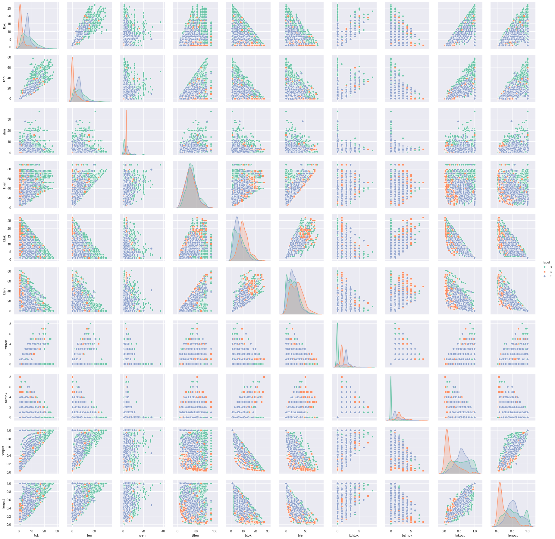
It is very likely that we cannot find the covariance of boolean features. So we do not include them in the correlogram above. The diagonal of the correlogram are histograms of a single feature against the label, whereas the off-diagonal ones are scatter plots of two features. Therefore we can read from the diagonal whether a feature is discriminative to the classification, also from off-diagonal whether a label is clustered by some features.
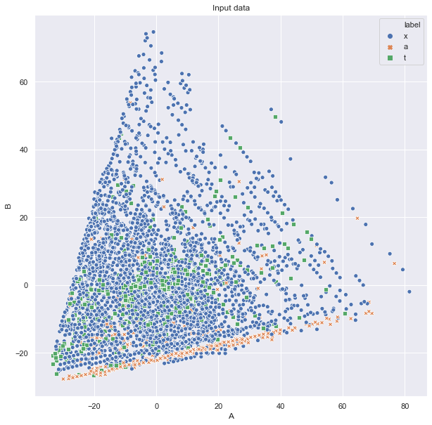
Then we can ask, whether there are some simple linear combination of features to be discriminative. We can do this based on principal component analysis and plot in 2D:
from sklearn.decomposition import PCA
import matplotlib.pyplot as plt
import seaborn as sns

pca = PCA(n_components=2)
pca.fit(df[incol])

plt.figure(figsize=(10,10))
ax = sns.scatterplot(data=pd.DataFrame(pca.transform(df[incol]), columns=["A","B"]).assign(label=df["label"]),
                     hue="label", style="label", x="A", y="B")
ax.set_title("Input data")
plt.show()
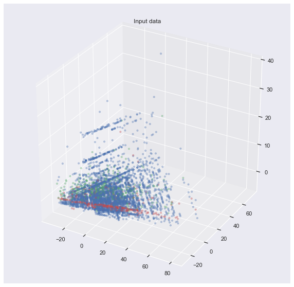
or even 3D:
from sklearn.decomposition import PCA
import matplotlib.pyplot as plt
from mpl_toolkits.mplot3d import Axes3D
import seaborn as sns

pca = PCA(n_components=3)
pca.fit(df[incol])

fig = plt.figure(figsize=(10, 10))
ax = fig.add_subplot(111, projection='3d')
xyz = pd.DataFrame(pca.transform(df[incol]), columns=["X","Y","Z"])
color = df["label"].replace({'a':'r', 't':'g', 'x':'b'})
ax.scatter(xyz["X"], xyz["Y"], xyz["Z"], c=color, s=10, alpha=0.3)
ax.set_title("Input data")
plt.show()
It is not so easy to show the decision boundary of each classifier. In fact, I don’t know how to visualize that. My attempt would be to use the axes produced by PCA and map the decision boundary onto it. But this is not beautiful:
#
# Prepare for plotting using PCA axes
#

X = df[incol]
y = df['label']

pca = PCA(n_components=2)
pca.fit(X)

# get size limit of input data, for plotting purpose
Xpca = pca.transform(X)
x_min, x_max = Xpca[:, 0].min() - .5, Xpca[:, 0].max() + .5
y_min, y_max = Xpca[:, 1].min() - .5, Xpca[:, 1].max() + .5

# generate input attributes
ranges = []
for c in incol:
    if c in numcols:  # numeric cols
        ranges.append(np.linspace(df[c].min(), df[c].max(), 10))
    else:  # boolean cols
        ranges.append(np.linspace(0, 1, 2))

# memory-save way to generate some data points to plot contour
griddf = pd.DataFrame([[np.random.choice(x) for x in ranges] for _ in range(5*N*N)], columns=incol)
gridpca = pca.transform(griddf)

# build a meshgrid according to input attributes. This will take a while
xx, yy = np.meshgrid(np.linspace(x_min, x_max, N), np.linspace(y_min, y_max, N))
zindex = np.ndarray(xx.shape, dtype=int)
for index in np.ndindex(*xx.shape):
    dist = np.linalg.norm(gridpca - np.array([xx[index], yy[index]]), axis=1)
    zindex[index] = np.argmin(dist)

# Create plot helper
def plot(X, y, axis, title, **kwargs):
    "Plot PCA-ized X over label Y in 2D scatter plot"
    ax = sns.scatterplot(data=pd.DataFrame(pca.transform(X), columns=["A","B"]).assign(label=y),
                         hue="label", style="label", x="A", y="B", ax=axis, **kwargs)
    ax.set_title(title)
    ax.set(xlim=(x_min, x_max), ylim=(y_min, y_max))

#
# Train, evaluate, and plot
#

cm = plt.cm.RdBu
f, axes = plt.subplots(4, 3, figsize=(21, 28))  # 3 col x 4 rows
axes = axes.ravel()  # unroll this into row-major 1D array
i = 0

# plot full input dataset
plot(X, y, axes[i], "All data", legend="brief")

# preprocess dataset, split into training and test part
X_train, X_test, y_train, y_test = train_test_split(X, y, test_size=.4, random_state=42)

# Plot the test set
i += 1
plot(X_test, y_test, axes[i], "Test", legend=None)

# iterate over classifiers and plot each of them
for name, clf in classifiers:
    i += 1
    i += 1
    # train and print report
    clf.fit(X_train, y_train)
    score = clf.score(X_test, y_test)
    print("\n----\n{} (score={:.5f}):".format(name, score))
    print(classification_report(y, clf.predict(X), digits=5))

    # Plot the decision boundary. For that, we will assign a color to each
    # point in the mesh [x_min, x_max]x[y_min, y_max].
    try:
        if hasattr(clf, "decision_function"):
            Z = clf.decision_function(griddf)[:, 1]
        else:
            Z = clf.predict_proba(griddf)[:, 1]

        # Put the result into a color plot
        zz = np.zeros(xx.shape)
        for index in np.ndindex(zindex.shape):
            zz[index] = Z[zindex[index]]
        axes[i].contourf(xx, yy, zz, cmap=cm, alpha=.8)

        # Plot the training points
        plot(X_train, y_train, axes[i], name, legend=None)
        plot(X_test, y_test, axes[i], name, legend=None, alpha=0.6)
        axes[i].text(x_max-.3, y_min+.3, '{:.2f}'.format(score).lstrip('0'),
                     size=15, horizontalalignment='right')
    except:
        pass # doesn't matter if error

plt.tight_layout()
plt.show()
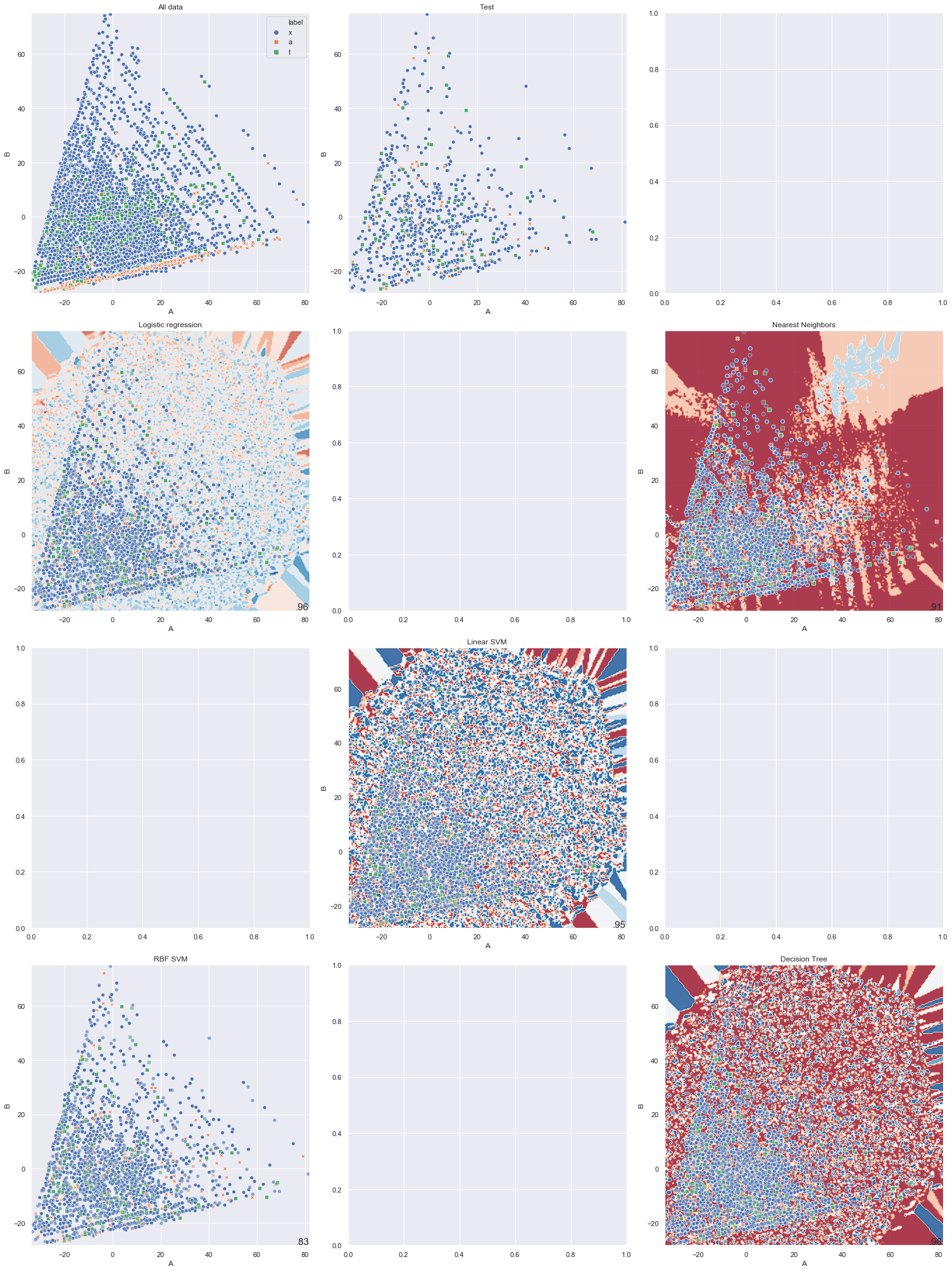
As we can see in the above graph, some classifier is quite messy and some other can’t even produce the contour. I am still looking for the right way to visualize this.
The Jupyter notebook for all the above is here.