Linear regression assumes a set of coordinates \((x_i, y_i),\ i=1,\cdots,N\) fits the relation
\[\begin{align} y &= \beta_0 + \beta_1 x + \epsilon \\ E[y|x] &= \beta_0 + \beta_1 x \end{align}\]which the error term \(\epsilon\) should be i.i.d. normally distributed with zero mean.
In general, with one dependend variable \(y_{i}\) and various independent variable \(x_{ji}\), we can define the linear regression model as
\[\begin{align} \mathbf{y} &= \mathbf{X}\mathbf{b} + \mathbf{e} \\ \textrm{where}\qquad \mathbf{y} &= \begin{bmatrix}y_1 & y_2 & \cdots & y_n\end{bmatrix}^T \\ \mathbf{X} &= \begin{bmatrix}\mathbf{x}_1 \\ \mathbf{x}_2 \\ \vdots \\ \mathbf{x}_n\end{bmatrix} = \begin{bmatrix} 1 & x_{11} & \cdots & x_{1p} \\ 1 & x_{21} & \cdots & x_{2p} \\ \vdots & \vdots & & \vdots \\ 1 & x_{n1} & \cdots & x_{np} \end{bmatrix} \\ \mathbf{b} &= \begin{bmatrix}\beta_0 & \beta_1 & \cdots & \beta_p \end{bmatrix}^T \\ \mathbf{e} &= \begin{bmatrix}\epsilon_0 & \epsilon_1 & \cdots & \epsilon_n \end{bmatrix}^T \end{align}\]or further make this into GLM by considering \(\mathbf{y}\) a \(q\)-column matrix instead of column vector, which \(\mathbf{b}\) and \(\mathbf{e}\) are also matrices of coefficient and error terms correspondingly.
The solution to simple linear model, \(\mathbf{y} = \mathbf{X}\mathbf{b} + \mathbf{e}\), using ordinary least square (OLS) is
\[\begin{align} \hat{\mathbf{b}} &= \arg\min \|\mathbf{X}\mathbf{b} - \mathbf{y} \|_2 \\ & = (\mathbf{X}^T\mathbf{X})^{-1}\mathbf{X}^T\mathbf{y} = \frac{1}{\sum_i\mathbf{x}_i\mathbf{x}_i^T} \sum_i \mathbf{x}_iy_i \end{align}\]which is obtained by evaluating the derivative of the above norm term equals to zero.
The variance estimator is proportional to variance of \(\epsilon\)
\[\mathrm{Var}(\hat{\mathbf{b}}) = \sigma^2 (\mathbf{X}^T\mathbf{X})^{-1}\]This is called the variance-covariance matrix and the standard error (used in the t-tests below) on the diagonal.
Although in the above, we have multiple indepdent variables \(x_{ji}\), in practice they can be correlated to each other. For example, by setting \(x_{ki} = x_{1i}^k\) for \(k>1\), we convert a linear regression model into a \(k\)-order polynomial regression model.
The simplest form for linear regression model is \(p=1\), which we only have coefficients \(\beta_0,\beta_1\) and each data point is a ordered pair \((x_i,y_i)\). The solution would be
\[\begin{align} \begin{bmatrix}\beta_0 \\ \beta_1\end{bmatrix} &= \begin{bmatrix}n & \sum_i x_i \\ \sum_i x_i & \sum_i x_i^2 \end{bmatrix}^{-1} \begin{bmatrix}\sum_i y_i \\ \sum_i x_i y_i \end{bmatrix} = \begin{bmatrix}n & n\bar{x} \\ n\bar{x} & \sum_i x_i^2 \end{bmatrix}^{-1} \begin{bmatrix}n\bar{y} \\ \sum_i x_i y_i \end{bmatrix} \\ &= \frac{1}{n\sum_i x_i^2 - n^2 \bar{x}^2} \begin{bmatrix}\sum_i x_i^2 & -n\bar{x} \\ -n\bar{x} & n \end{bmatrix} \begin{bmatrix}n\bar{y} \\ \sum_i x_i y_i \end{bmatrix} \\ &= \begin{bmatrix} \dfrac{\bar{y}\sum_i x_i^2 - \bar{x}\sum_i x_i y_i}{\sum_i x_i^2 - n\bar{x}^2} \\ \dfrac{\sum_i x_i y_i - n \bar{x}\bar{y}}{\sum_i x_i^2 - n \bar{x}^2} \end{bmatrix} = \begin{bmatrix} \dfrac{\bar{y}\sum_i x_i^2 - \bar{x}\sum_i x_i y_i}{\sum_i (x_i - \bar{x})^2} \\ \dfrac{\sum_i (x_i-\bar{x})(y_i-\bar{y})}{\sum_i (x_i - \bar{x})^2} \end{bmatrix} \end{align}\]Such solution is in the sense that provides the BLUE — best linear unbiased estimator of the form \(y=\beta_0 + \beta_1 x.\) We consider only this type of linear regression model below, with the notation \(\hat{y}_i = \hat{\beta}_0 + \hat{\beta}_1 x_i\)
Now the question is how well this estimator is given a particular set of input. It turns out there are different ways to answer this.
(1) Is there a linear relationship between \(x\) and \(y\)?
If so, it should be \(\beta_1\ne 0\). In general we can ask if \(\beta_1 \ne \beta_1^{\ast}\) for some known \(\beta_1^{\ast}\) derived from some hypothesis. In this case the t test is handy, which use the test statistic1
\[\begin{align} T &= \frac{\hat{\beta}_1 - \beta_1^{\ast}}{SE(\hat{\beta}_1)} \\ \textrm{where}\qquad SE(\hat{\beta}_1) &= \sqrt{\frac{1}{n-2}\frac{\sum_i (y_i - \hat{y}_i)^2}{\sum_i (x_i-\bar{x})^2}} = \sqrt{\frac{1}{n-2}\frac{\sum_i \hat{\epsilon}_i^2}{\sum_i (x_i-\bar{x})^2}} \end{align}\]which \(T\) should follow t-distribution with \(n-2\) df under the null hypothesis (i.e. \(\hat{\beta}_1 = \beta_1^{\ast}\)). We can test if \(T\) falls between \(\pm t_{\alpha/2,n-2}\).
(2) Is the intercept \(\beta_0\) significant?
Similarly, we can use the t test with statitics2
\[\begin{align} T &= \frac{\hat{\beta}_0 - \beta_0^{\ast}}{SE(\hat{\beta}_0)} \\ \textrm{where}\qquad SE(\hat{\beta}_0) &= \sqrt{\frac{1}{n(n-2)}\sum_i\hat{\epsilon}_i^2\frac{\sum_i x_i^2}{\sum_i (x_i-\bar{x})^2}} \end{align}\]A side note: Given the confidence level \(\alpha\) and SE of \(\hat{\beta}_0\) and \(\hat{\beta}_1\), we can use t-distribution to derive the confidence interval of each coefficient and model output
\[\begin{align} \hat{\beta}_0 & \pm t_{\alpha/2,n-2} SE(\hat{\beta}_0) \\ \hat{\beta}_1 & \pm t_{\alpha/2,n-2} SE(\hat{\beta}_1) \\ \hat{y}_i & \pm t_{\alpha/2,n-2} \sqrt{ \hat{\sigma}^2\left( \frac{1}{n}+\frac{(x_i-\bar{x})^2}{\sum_j(x_j-\bar{x})^2} \right) } \\ & \textrm{where}\ \hat{\sigma}^2 = \frac{1}{n-2}\sum_i\hat{\epsilon}_i^2 \end{align}\]Because the SE decreases as \(n\) increases, we can applying this reversely to check if (but not easy to derive due to dependency of variation of inputs \(x_i\)) the sample size \(n\) is large enough given the error margin of \(y_i\) and confidence level \(\alpha\).
(3) How accurate is the regression fit the data?
This is asking if the distribution of data is really what the regresion describes. To check if a model fits data, we use ANOVA. We define
- Total sum of square: \(TSS = \sum_i (y_i - \bar{y})^2\)
- Regression sum of square: \(RSS = \sum_i (\hat{y}_i - \bar{y})^2\)
- Error sum of square: \(ESS = \sum_i (y_i - \hat{y}_i)^2\)
and then \(TSS = RSS + ESS\). The RSS, with df of 1, explains the variability of \(\hat{y}_i\) due to variability of input \(x_i\). ESS, with df of \(n-2\) is the remaining variability not explained by the regression model, which \(\hat{\sigma}^2 = ESS/(n-2)\) is the estimator for the variation of \(\epsilon\). The total variability TSS has a df of \(n-1\).
We can then use the F-test3 with statistic
\[F' = \frac{RSS/1}{ESS/(n-2)} = \frac{RSS}{\hat{\sigma}^2}\]against the F-distribution with df \((1,n-2)\). The linear model is a good fit if \(F' < F_{\alpha, 1, n-2}\) or equivalently the \(p\)-value of the linear model is given by
\[p = 1- \Pr[F_{1,n-2}(x) < F']\]Indeed, a related measure is the coefficient of determination \(R^2\), defined as
\[R^2 = \frac{RSS}{TSS} = \frac{\sum_i (\hat{y}_i - \bar{y})^2}{\sum_i (y_i-\bar{y})^2} \in [0,1]\]which accounts for the proportion of variability in data explained by the regression model. A good fit if \(R^2\to 1\).
Interpreting Julia’s GLM package
As an example, we will see the abovementioned metrics from any statistical packages, such as GLM in Julia.
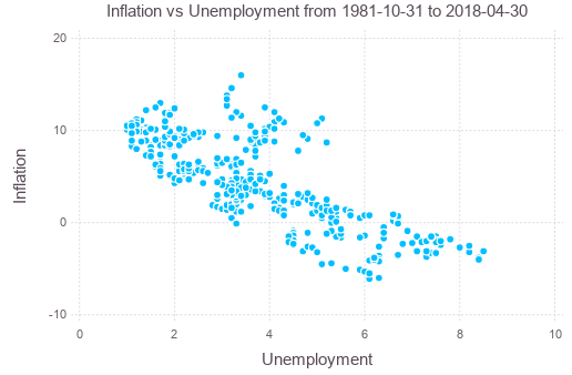
Consider the Phillips curve, namely, the empirical model that unemployment and inflation are correlated (Milton Friedman’s interpretation). To show how accurate is this hypothesis, we check the linear regression model between inflation rate (based on CPI, YoY) and unemployment rate. Trading Economics has these data since 1981.
After downloading the data in CSV format, we can read them into data frame, join them and plot:
using CSV
using DataFrames
using Gadfly

cpi = CSV.read("hkcpiy.csv", header=["Date","Inf"], footerskip=2, datarow=2, allowmissing=:none)
ue = CSV.read("hkuerate.csv", header=["Date","UE"], footerskip=2, datarow=2, allowmissing=:none)
phillips = join(cpi, ue, on=:Date, kind=:inner)
plot(phillips, x=:UE, y=:Inf, Geom.point,
     Guide.XLabel("Unemployment"), Guide.YLabel("Inflation"),
     Guide.Title("Inflation vs Unemployment from "
                 * string(minimum(cpi[:Date])) * " to " * string(maximum(cpi[:Date])))
    )
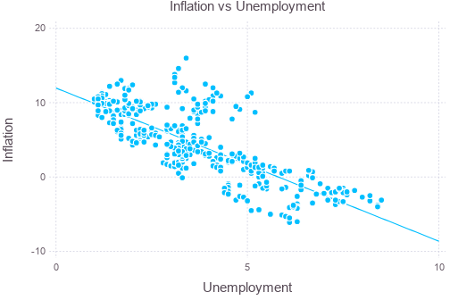
Perform linear regression (ordinary least square method) against the data, and plot the regression result:
using GLM
ols = lm(@formula(Inf ~ UE), phillips)
intercept = coef(ols)[1]
slope = coef(ols)[2]
xx = collect(0:0.1:10)
yy = intercept + xx*slope
plot(layer(phillips, x=:UE, y=:Inf, Geom.point),
     layer(x=xx, y=yy, Geom.line),
     Guide.XLabel("Unemployment"), Guide.YLabel("Inflation"),
     Guide.Title("Inflation vs Unemployment"))
The function call lm() will print the following into the console:
Formula: Inf ~ 1 + UE

Coefficients:
             Estimate Std.Error  t value Pr(>|t|)
(Intercept)    11.961  0.332921  35.9274   <1e-99
UE           -2.05903 0.0822117 -25.0454   <1e-85
The estimate column above are coefficients of the constant term and the unemployment rate variable (i.e., \(\hat{\beta}_0, \hat{\beta}_1\)). It suggests that the inflation \(I\) and unemployment \(U\) are related as \(I=11.961-2.05903U\). The std error column is the numerical values of \(SE(\hat{\beta}_0),SE(\hat{\beta}_1)\). The t value column is for \(\beta_0^{\ast}=\beta_1^{\ast}=0\) and represents the test statistic \(T=\hat{\beta}_i/SE(\hat{\beta}_i)\). Finally, the probability column shows the confidence level \(\alpha\) corresponding to the t value. Such value suggests that there is very strong correlation between the two.
\(R^2\) is given by r2(ols), which gives the result 0.5893907142373523. From
this we see there is quite significant noise that is not covered by the model.
In this exercise, we are using 439 data points. If we limit the data to, say, last 10 years, the GLM result will give a much weaker \(R^2\), greater std error, smaller t value, and lower confidence level, even though the correlation is still established.
-
Wikipedia article on Student’s t-test ↩
-
Wikipedia article on simple linear regression ↩
-
F-test accounts for the ratio between two chi-distributions ↩