Artificial Neural Network using only numpy

I know there are tensorflow, pytorch, kera and a whole bunch of other libraries out there but I need something that can work on Termux but no success (at least no longer after Python 3.7 upgrade). But after reading again the textbook on how a neural network operates, it doesn’t seem hard to write my own library.

Here I explain the code:

Symbols and notations

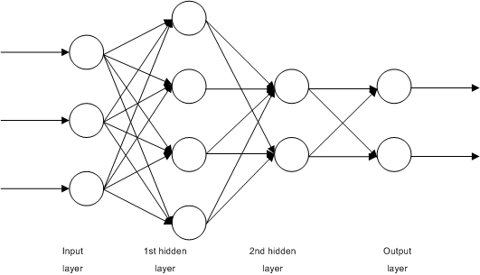
Artificial neural network is a non-linear regression model in stacked layers. The simple regression in statistics is having one input and one output and to find the equation to fit in between. A multilayer neural network (MLP, multilayer perceptron) is to extend this structure to multiple layers, so regression on layer \(n\) gives output that will become input of the layer \(n+1\). Input to layer 0 is the model’s input and the output from the last layer is the model’s output.

Using a notation similar to Russell and Norvig’s book ¹, we can model the NN as follows:

• there are \(N\) layers in the NN
• model input is matrix \(\mathbf{X}\), which the convention is to have features of each data point as rows, and different data are presented as columns. We will have \(m\times n\) matrix for \(n\) instances of data, each having \(m\) features
• model reference output is matrix \(\mathbf{Y}\), which again, data of each instances are presented as columns. We will have \(r\times n\) matrix for the same \(n\) instances of data, each having \(r\) output features
• \(\mathbf{A}^{(\ell)}\) is the input of layer \(\ell\) and output of layer \(\ell-1\). It will be a matrix of dimension \(s\times n\) if there are \(s\) perceptrons on layer \(\ell-1\)
• \(\mathbf{A}^{(0)} = \mathbf{X}\) by definition, and we define the model output \(\hat{\mathbf{y}} = \mathbf{A}^{(N)}\)

• each perceptron (building block of NN) computes \(z = \mathbf{w}^T\mathbf{a} + b\) for some weight vector \(\mathbf{w}\) and the input to the layer \(\mathbf{a}\) for each instance of data, then outputs \(g(z)\) for some activation function \(g()\). This is the non-linear function in the regression. In matrix form for all instances of data and the whole layer on layer \(\ell\), it is

  \[\mathbf{A}^{(\ell)} = g(\mathbf{Z}^{(\ell)}) = g(\mathbf{W}^{(\ell)}\mathbf{A}^{(\ell-1)} + \mathbf{b})\]

  where the addition of \(\mathbf{b}\) above is broadcast to each row. Matrix \(\mathbf{W}^{(\ell)}\) is of dimension \(r\times s\) for this layer has \(r\) perceptrons and the previous layer has \(s\) perceptrons. Matrices \(\mathbf{A}^{(\ell)}\) and \(\mathbf{A}^{(\ell-1)}\) is of dimensions \(r\times n\) and \(s\times n\) respectively

• The activation function \(g()\) is commonly one of these:
  • ReLU \(g(z) = \max(0, z)\)
  • logistic: \(g(z) = \frac{1}{1+e^{-z}}\)
  • hyperbolic tangent: \(g(z) = \tanh(z)=\frac{e^z - e^{-z}}{e^z + e^{-z}}\)
  • leaky ReLU: \(g(z) = az\) for some small \(a>0\) when \(z<0\) otherwise \(g(z)=z\)
  • ELU: \(g(z) = a(e^z-1)\) for some small \(a>0\) when \(z<0\) otherwise \(g(z)=z\)

To train the NN, we feed forward the network with data \(\mathbf{X}\) and \(\mathbf{Y}\) in each epoch and then use back propagation to update the parameters, then repeat for many epochs in the hope that the parameters will converge to a useful value. First we define a loss function \(L(\mathbf{Y}, \hat{\mathbf{Y}})\) to measure the average discrepancy between the NN output \(\hat{\mathbf{Y}}\) and the reference output \(\mathbf{Y}\) over the \(n\) data instances. Then we minimize \(L\), usually by gradient descent method: On output layer:

Otherwise:

which the sum on \(d\mathbf{b}^{(\ell)}\) is to sum on all columns of \(d\mathbf{Z}^{(\ell)}\). Then we update the parameters by

For some learning rate \(\alpha\). Observing the definition of each differentials, they are all partial derivatives of \(L\) w.r.t. each parameters to update. Hence the above two equations as update rule. It is common to use binary cross entropy as loss function for classification applications: (in scalar form)

which then we have

How to use it

Sample code:

from pyann import pyann

# make N instances of data stacked as columns of numpy array
X, y = prepare_data()
X_train, X_test, y_train, y_test = train_test_split(X, Y)

# learn it
layers = [2, 50, 50, 50, 1]
activators = ["relu"] * 4 + ["logistic"]
NN = pyann(layers, activators)
NN.fit(X_train, y_train, 10000, 0.001, printfreq=500)

# use it
y_hat = NN.forward(X_test)

What can go wrong

The recent O’Reilly book² has a very well-written Chapter 11. I would say, all problems it describes can happen to this code. So you cannot use it to build a deep neural network out of the box.

First is the issue of vanishing gradients and exploding gradients. The problem will be exaggerated when the network has a lot of layers. The code above did not implement Xavier initialization (just very simple quasi-truncated normal).

Second is the saturation of the ReLU activation functions. It is common to use ReLU, and it may saturate to its flattened region (negative \(Z\)) that render the NN malfunction. We did not implement leaky ReLU above, but we do have the exponential linear unit (ELU) with parameter 1 to the rescue. But using it will see noticeable slow down.

Third, no regularization and no early stopping is implemented. After all, we have no way to provide test set to the NN model to fit.

Lastly, we did not implement drop out. I heard people do not use it any more in favor of other techniques. But if you want to, we have to implement masks to the weight matrices \(W\).

Except that it is simple, usable, and not depend on sophisticated libraries, this is far from a feature-rich NN framework. Try at your own risk.