Solving equations using Tensorflow 2 and PyTorch

Consider the following problem of 4 linear equations and 4 unknowns:

[ A ]  +  [ B ]  =  8
  +         +
[ C ]  -  [ D ]  =  6
  =         =
  13        8

The simplest way to solve such simultaneous equations is to use sympy:

import sympy
A, B, C, D = sympy.symbols("A B C D")
sympy.linsolve([
    A+B-8,
    A+C-13,
    C-D-6,
    B+D-8,
], (A, B, C, D))

The sympy.linsolve() call above will produce the following set of single solution, i.e., a unique solution is found for this:

{(7/2, 9/2, 19/2, 7/2)}

But for many cases of similar type, we can also approach the problem with an iterative solution. If we think about it, the gradient descent is indeed an iterative solution technique. So if we try to solve the same problem with TensorFlow 2, with initial solution of all zero, and use squared error as the loss function, we can do this:

import tensorflow as tf
import matplotlib.pyplot as plt

# Define a model
A = tf.Variable(0.0, name='A')
B = tf.Variable(0.0, name='B')
C = tf.Variable(0.0, name='C')
D = tf.Variable(0.0, name='D')

def loss(A, B, C, D):
  resP8 = tf.add(A, B, name="A+B")
  resQ6 = tf.subtract(C, D, name="C-D")
  resR13 = tf.add(A, C, name="A+C")
  resS8 = tf.add(B, D, name="B+D")
  return tf.square(8.0 - resP8) + tf.square(6.0 - resQ6) + tf.square(13.0 - resR13) + tf.square(8.0 - resS8)

def train(learning_rate):
  with tf.GradientTape() as t:
    current_loss = loss(A, B, C, D)
    dA, dB, dC, dD = t.gradient(current_loss, [A, B, C, D])
  A.assign_sub(learning_rate * dA)
  B.assign_sub(learning_rate * dB)
  C.assign_sub(learning_rate * dC)
  D.assign_sub(learning_rate * dD)

# Collect the history of values to plot later
As, Bs, Cs, Ds = [], [], [], []
N = 30
for epoch in range(N):
  As.append(A.numpy())
  Bs.append(B.numpy())
  Cs.append(C.numpy())
  Ds.append(D.numpy())
  current_loss = loss(A, B, C, D)
  train(learning_rate=0.25)
  if epoch % (N//10) == 0 or epoch == N-1:
    print('Epoch %2d: A=%1.2f B=%1.2f, C=%1.2f, D=%1.2f, loss=%2.5f' %
          (epoch, As[-1], Bs[-1], Cs[-1], Ds[-1], current_loss))

# Let's plot it all
epochs = list(range(N))
plt.plot(epochs, As, 'r',
         epochs, Bs, 'b',
         epochs, Cs, 'c',
         epochs, Ds, 'g')
plt.legend(['A', 'B', 'C', 'D'])
plt.show()

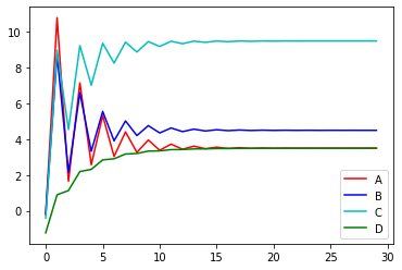
The solution is close enough at merely 15 epochs, and the following is the chart of convergence, note the solution is \((A,B,C,D) = (3.5, 4.5, 9.5, 3.5)\)

Similarly, we can use PyTorch to do the same. We can see that the code are indeed quite similar:

import torch
import matplotlib.pyplot as plt

dtype = torch.float
device = torch.device("cpu")  # or "cuda:0"

# Define a model
A = torch.randn(1, 1, device=device, dtype=dtype, requires_grad=True)
B = torch.randn(1, 1, device=device, dtype=dtype, requires_grad=True)
C = torch.randn(1, 1, device=device, dtype=dtype, requires_grad=True)
D = torch.randn(1, 1, device=device, dtype=dtype, requires_grad=True)

def loss(A, B, C, D):
  resP8 = A+B
  resQ6 = C-D
  resR13 = A+C
  resS8 = B+D
  return (8.0 - resP8)**2 + (6.0 - resQ6)**2 + (13.0 - resR13)**2 + (8.0 - resS8)**2

def train(learning_rate):
    global A, B, C, D
    current_loss = loss(A, B, C, D)
    current_loss.backward()
    with torch.no_grad():
        A -= learning_rate * A.grad
        B -= learning_rate * B.grad
        C -= learning_rate * C.grad
        D -= learning_rate * D.grad
        # Reset gradient
        A.grad.zero_()
        B.grad.zero_()
        C.grad.zero_()
        D.grad.zero_()

# Collect the history of values to plot later
As, Bs, Cs, Ds = [], [], [], []
N = 30
for epoch in range(N):
  As.append(float(A.detach().numpy()))
  Bs.append(float(B.detach().numpy()))
  Cs.append(float(C.detach().numpy()))
  Ds.append(float(D.detach().numpy()))
  current_loss = loss(A, B, C, D)
  train(learning_rate=0.25)
  if epoch % (N//10) == 0 or epoch == N-1:
    print('Epoch %2d: A=%1.2f B=%1.2f, C=%1.2f, D=%1.2f, loss=%2.5f' %
          (epoch, As[-1], Bs[-1], Cs[-1], Ds[-1], current_loss))

# Let's plot it all
epochs = list(range(N))
plt.plot(epochs, As, 'r',
         epochs, Bs, 'b',
         epochs, Cs, 'c',
         epochs, Ds, 'g')
plt.legend(['A', 'B', 'C', 'D'])
plt.show()

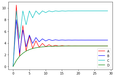
The following shows the rate of convergence. I would say there is no obvious difference from that of TensorFlow.