Jupyter notebooks and visualization are natural marriage. It is more fun if we can skew this or that a bit by turning a knob or selecting something from a drop down. This is where so called interactive widgets come to play. There are a lot of examples on how to set up a widget and control the matplotlib chart interactively. Doing so in jupyterlab, however, is not so straightforward.
matplotlib and the widgets
Jupyter notebook widgets are just come control elements for user interaction. They receive user input and trigger events, which then can invoke some function. To use widgets to control matplotlib graphics, we have to understand what are the matplotlib backends.
%matplotlib --list
This, if run in jupyter, will list out all backends. In my case,
Available matplotlib backends: ['tk', 'gtk', 'gtk3', 'wx', 'qt4', 'qt5', 'qt',
'osx', 'nbagg', 'notebook', 'agg', 'svg', 'pdf', 'ps', 'inline', 'ipympl',
'widget']
Amongst them the inline backend is the dumbest. Which just render the plot
and make it read-only. Therefore, no update is allowed on the chart, but you
can always clear it and redraw. The notebook backend makes the matplotlib
output aware of the Jupyter environment and the charts can be updated. The
widget and ipympl backend are similar to that of notebook, but fancier.
They make the matplotlib output as a widget that you can pan or zoom. Using
matplotlib with different backend requires the interactive widgets to be
configured differently.
The widgets on jupyter is from the module ipywidgets. The simplest example (without graphics!) is as follows:
from ipywidgets import interact
def f(x):
return x**2
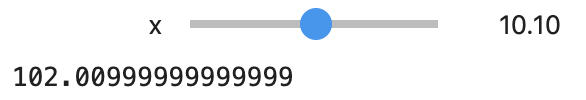
interact(f, x=10.0);
Running this in a jupyter notebook will give you a slider and a row of text (for printing the output of the function):
a equivalent way of the above would be the following snippet, which use interact() as a decorator:
from ipywidgets import interact, widgets
@interact(x=widgets.FloatSlider(min=-10, max=30, step=0.1, value=10))
def f(x):
    return x**2
The interact() decorator accepts keyword arguments that match with the
function. You may create the widget explicitly and assign to the keyword
argument, or in a short form, you can also simply provide a value and let
interact() infer the widget. If the argument is:
- a boolean (
TrueorFalse), a checkbox widget is provided (widgets.Checkbox) - an integer or a float: a slider widget is provided (
widgets.IntSliderorwidgets.FloatSlider) - a string: a textbox widget is provided (
widget.Text) - a list of strings: a dropdown widget is provided (
widget.Dropdown)
Full list of available widgets and their configuration can be found in ipywidget documentation
The way to connect the ipywidgets to matplotlib is as follows.
Let us try to plot a sine curve with different angular frequency, phrase, and
amplitude. If we use the inline backend, this is the code:
import numpy as np
import matplotlib.pyplot as plt
from ipywidgets import interact
%matplotlib inline

x = np.linspace(0, 5*np.pi, 500)

@interact(w=(0, 10, .1), amp=(-4, 4, .1), phi=(0, 2*np.pi, 0.1))
def plot(w=1.0, amp=1, phi=0):
    y = amp*np.sin(w*x-phi)
    plt.plot(x,y)
	plt.ylim([-4,4])
    plt.show()
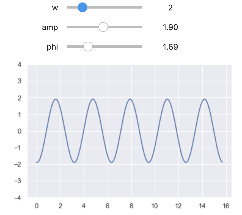
The function plot() uses keyword arguments that matched the interact()
function. The tuple notations are just another way to specify a slider (in
terms off min, max, and step). In the function, it simply replot the figure
everytime using the value provided by the slider. This works in inline
backend because all pictures are static.
If we use the widget backend or ipympl backend instead, we do this:
%matplotlib widget
fig, ax = plt.subplots(figsize=(6, 4))
ax.set_ylim([-4, 4])
ax.grid(True)

# fix x values
x = np.linspace(0, 5*np.pi, 500)
ax.scatter(x[::20], np.cos(x)[::20], color='r', alpha=0.5)

@interact(w=(0, 10, .1), amp=(-4, 4, .1), phi=(0, 2*np.pi, 0.1))
def update(w=1.0, amp=1, phi=0):
    """Remove old lines from plot and plot new one"""
    for l in ax.lines:
        l.remove()
    ax.plot(x, amp*np.sin(w*x-phi), color='C0')
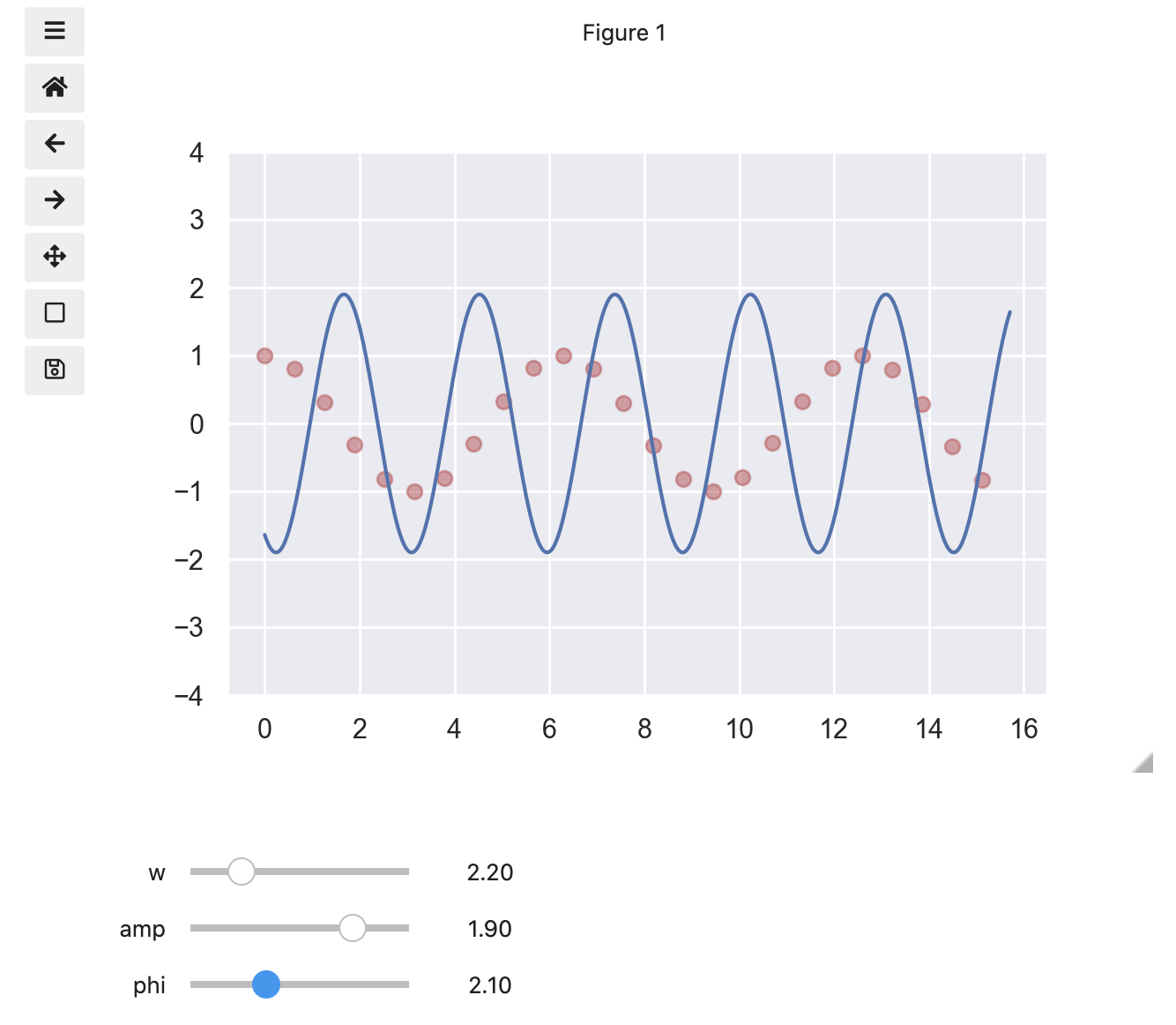
This is different from the previous in the sense that we do not call
plt.show() but simply remove the plot line and draw a new one. Note that when
we do the removal, the scatter plot is not removed because it is not part of
the ax.lines. Also, we do not need to redraw other elements of the plot. The
figure about also shows the icons on the left, which are part of the widget
or ipympl backend that allows us to pan and zoom.
There is yet another way to do the same, which the line is not even removed but simply updated:
%matplotlib notebook
fig, ax = plt.subplots(figsize=(6, 4))
ax.set_ylim([-4, 4])
ax.grid(True)

# fix x values, and create line plot object
x = np.linspace(0, 5*np.pi, 500)
line, = ax.plot(x,np.sin(x))

@interact(w=(0, 10, .1), amp=(-4, 4, .1), phi=(0, 2*np.pi, 0.1))
def plot(w=1.0, amp=1, phi=0):
    line.set_ydata(amp*np.sin(w*x-phi))
	#fig.canvas.draw()
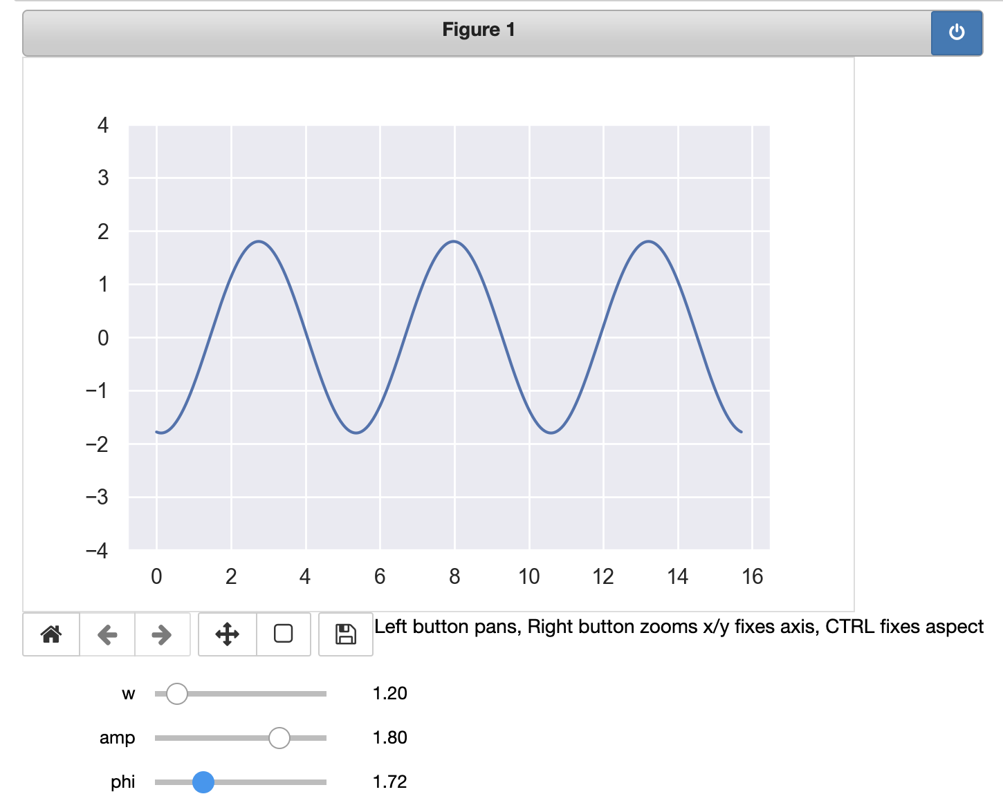
This code works only on jupyter-notebooks but not jupyterlab, for the
notebook backend is used. What it does is to create a line as a object from
ax.plot() and then when the widgets are updated, the data of the line are
updated using line.set_ydata(). Usually you may see the examples elsewhere
would invoke fig.canvas.draw() after the set_ydata() function so the
changes are applied. But I found that is unnecessary.
If we use seaborn, the code is mostly the same since it is just a wrapper to
matplotlib. The exception is the line object in the notebook backend example
above as seaborn.lineplot() will return you the axis, not the line object.
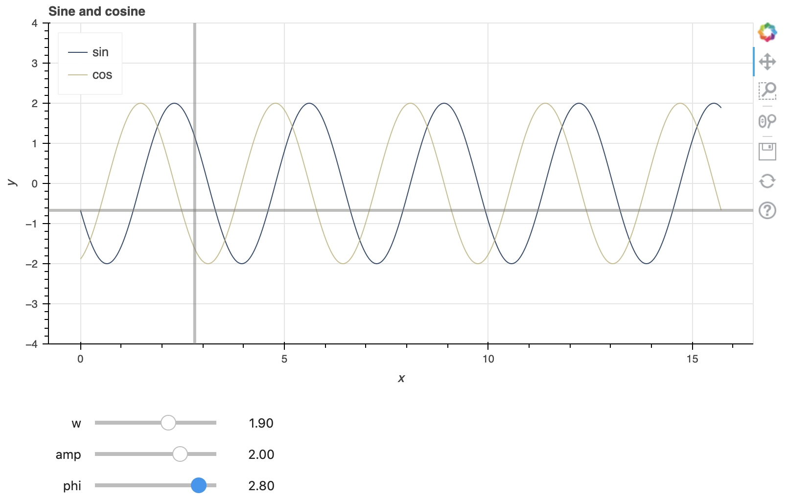
Bokeh and ipywidget
This is a similar example in Bokeh
from bokeh.io import output_notebook, push_notebook
output_notebook()

from bokeh.layouts import column, row
from bokeh.models import Slider, Span, Range1d
from bokeh.plotting import figure, show
from bokeh.palettes import cividis

from ipywidgets import interact, interactive, widgets

plot = figure(plot_width=800, plot_height=400)
x = np.linspace(0, 5*np.pi, 500)
color = cividis(5)
sine = plot.line(x, np.sin(x), line_width=1, alpha=0.8, line_color=color[0], legend_label="sin")
cosine = plot.line(x, np.cos(x), line_width=1, alpha=0.8, line_color=color[3], legend_label="cos")
vline = Span(location=0, dimension="height", line_color=color[2], line_width=3, line_alpha=0.5)
hline = Span(location=0, dimension="width", line_color=color[2], line_width=3, line_alpha=0.5)
plot.add_layout(vline)
plot.add_layout(hline)
plot.title.text = "Sine and cosine"
plot.legend.click_policy = "hide"
plot.legend.location = "top_left"
plot.xaxis.axis_label = "x"
plot.yaxis.axis_label = "y"
plot.y_range = Range1d(-4, 4)
handle = show(plot, notebook_handle=True)

# Slider: Using ipython widgets slider instead of Bokeh slider
@interact(w=widgets.FloatSlider(min=-10, max=10, value=1),
          amp=widgets.FloatSlider(min=-5, max=5, value=1),
          phi=widgets.FloatSlider(min=-4, max=4, value=0))
def update(w=1.0, amp=1, phi=0):
    sine.data_source.data["y"] = amp*np.sin(w*x-phi)
    cosine.data_source.data["y"] = amp*np.cos(w*x-phi)
    vline.location = phi
    hline.location = amp*np.sin(-phi)
    push_notebook(handle=handle)
The logic is similar to the case of notebook backend for matplotlib but this
works for both jupyter-notebooks and jupyterlab. Bokeh allows to change the
data of the data source but the x and y dimension must be consistent. If we
change the curve entirely, we can either use data_source.data.update(x=x, y=y)
to do the update in one shot, or reassign the data with data_source.data =
newdata, where newdata can be a python dictionary. What necessary in using
Bokeh interactively are
- after we set up the figure, we show it with
show(plot, notebook_handle=True)and remember the handle - in the update function, after we update the data, we need to invoke
push_notebook(handle=handle)to refresh the figure as pointed by the handle
The handle is not necessarily for one figure. Other widgets or multiple figures
can be shown using the same notebook handle. The push_notebook() call is to
make the handle refresh itself as some underlying data is known to be changed.
Bokeh indeed goes with its own slider widget but it will not work in the notebook because it is purely Javascript. Unless we can do the interactive update in Javascript (e.g., all data are loaded, and the updated value can be computed using Javascript), it will not get the job ddone. The other use of Bokeh widgets is when we have a Bokeh server, which the widget will get the data updated via a web request. If we use the Bokeh slider anyway, we will get an error message:
def update(w=1.0, amp=1, phi=0):
    sine.data_source.data["y"] = amp*np.sin(w*x-phi)
    cosine.data_source.data["y"] = amp*np.cos(w*x-phi)
    vline.location = phi
    hline.location = amp*np.sin(-phi)
    push_notebook(handle=handle)

# Bokeh sliders
slider_w = Slider(start=-10, end=10, value=1, step=0.1, title="frequency")
slider_amp = Slider(start=-5, end=5, value=1, step=0.1, title="amplitude")
slider_phi = Slider(start=-4, end=4, value=0, step=0.1, title="phrase")
def slider_change(attr, old, new):
    update(slider_w.value, slider_amp.value, slider_phi.value)
slider_w.on_change('value', slider_change)
slider_amp.on_change('value', slider_change)
slider_phi.on_change('value', slider_change)
handle = show(column(plot, slider_w, slider_amp, slider_phi), notebook_handle=True)
This will be shown on the notebook with the widgets impotent.
WARNING:bokeh.embed.util:
You are generating standalone HTML/JS output, but trying to use real Python
callbacks (i.e. with on_change or on_event). This combination cannot work.

Only JavaScript callbacks may be used with standalone output. For more
information on JavaScript callbacks with Bokeh, see:

    https://docs.bokeh.org/en/latest/docs/user_guide/interaction/callbacks.html

Alternatively, to use real Python callbacks, a Bokeh server application may
be used. For more information on building and running Bokeh applications, see:

    https://docs.bokeh.org/en/latest/docs/user_guide/server.html
Jupyterlab
Because of the different design, the jupyter notebook is way easier to set up
the interactive widgets. Your installation should include ipywidgets and
widgetsnbextension (which the latter should be automatically installed by the
former). To get the ipywidgets working in jupyterlab, after these python
modules are installed, you still need to install node.js (brew install
nodejs) and then run the following command
jupyter labextension install @jupyter-widgets/jupyterlab-manager
After this, a restart of jupyterlab will make it work.