Normalization in deep learning is to shift and scale a tensor such that the activation will run at the sweet spot. This helps to solve the problems such as vanishing/exploding gradients, weight initialization, training stability, and convergence.
Traditionally, a tensor in deep learning is in 4D and has the shape $(N,H,W,C)$ for the batch size, height, width, and channel respectively.
Batch Normalization was introduced to reduce the internal covariate shift, namely, the change in the distribution of the activation as the weight changed during training. It was known that training is faster if the inputs are whitened (i.e., $\mu=0, \sigma^2=1$, and decorrelated).
Batch normalization calculates the mean and variance of the input. In the case of convolution networks, the same convolution kernel is applied across the $H$ and $W$ dimension but separate on each $C$ dimension. Hence, in equation, the mean and variance are:
\[\begin{aligned} \mu_c &= \frac{1}{N}\frac{1}{H}\frac{1}{W} \sum_{n=1}^N \sum_{h=1}^H \sum_{w=1}^W x_{nhwc} \\ \sigma_c^2 &= \frac{1}{N}\frac{1}{H}\frac{1}{W} \sum_{n=1}^N \sum_{h=1}^H \sum_{w=1}^W (x_{nhwc} - \mu_c)^2 \end{aligned}\]Then the input is normalized to be:
\[\hat{x}_{nhwc} := \frac{x_{nhwc}-\mu_c}{\sqrt{\sigma_c^2+\epsilon}}\]and returns the output $y_{nhwc} = \gamma_c \hat{x}_{nhwc} + \beta_c$ for the parameters $\gamma_c,\beta_c$ to be learned. The returned tensor $\mathbf{y}$ shall have the same shape as the input tensor $\mathbf{x}$. Batch norm keeps the EWMA of the in-batch mean $\mu_c$ and in-batch variance $\sigma_c^2$ of input $\mathbb{x}$. At inference, together with the learned $\gamma_c$ and $\beta_c$, output was produced as
\[y_{nhwc} = \gamma_c \frac{x_{nhwc}-\mu_c}{\sqrt{\sigma_c^2+\epsilon}} + \beta_c = \frac{\gamma_c}{\sqrt{\sigma_c^2+\epsilon}} x_{nhwc} + \big(\beta_c - \frac{\gamma_c \mu_c}{\sqrt{\sigma_c^2+\epsilon}}\big)\]where $\mu_c$ and $\sigma_c^2$ are the EWMA calculated during training, expected to approximate $E[x]$ and $Var[x]$ over all training samples.
The accuracy of batch norm (specifically, the calculation of mean and variance) depends on a large enough batch size. Also, computing them in a recurrent network is difficult.
Layer Normalization performs across all channels and spatial dimensions. It is popularized only after the Transformer architecture use it. It simply computes the statistics over all units in the same layer, but the normalization term can be different in each training sample:
\[\begin{aligned} \mu_n &= \frac{1}{H}\frac{1}{W}\frac{1}{C} \sum_{h=1}^H \sum_{w=1}^W \sum_{c=1}^C x_{nhwc} \\ \sigma_n^2 &= \frac{1}{H}\frac{1}{W}\frac{1}{C} \sum_{h=1}^H \sum_{w=1}^W \sum_{c=1}^C (x_{nhwc}-\mu_n)^2 \\ \hat{x}_{nhwc} &= \frac{x_{nhwc}-\mu_n}{\sqrt{\sigma_n^2+\epsilon}} \\ y_{nhwc} &= \gamma_c \hat{x}_{nhwc} + \beta_c \end{aligned}\]The learnable weights $\gamma_c,\beta_c$ are channel-specific in Keras default implementation, but configurable. Since the mean and variance is calculated for each layer, there is no other parameter needed. To show this (in Keras) consider the following code:
import keras
bnlayer = keras.layers.BatchNormalization()
bnlayer.build([3,5,7,11])

lnlayer = keras.layers.LayerNormalization()
lnlayer.build([3,5,7,11])

print(bnlayer.get_config()["axis"])  # ListWrapper([3])
print(lnlayer.get_config()["axis"])  # ListWrapper([3])

print(bnlayer.weights)   # gamma, beta, moving_mean, moving_variance: all of shape (11,)
print(lnlayer.weights)   # gamma, beta: both of shape (11,)
An example implementation is found here:
class LayerNorm(nn.Module):
    """
    A LayerNorm variant, popularized by Transformers, that performs point-wise mean and
    variance normalization over the channel dimension for inputs that have shape
    (batch_size, channels, height, width).
    https://github.com/facebookresearch/ConvNeXt/blob/d1fa8f6fef0a165b27399986cc2bdacc92777e40/models/convnext.py#L119  # noqa B950
    """

    def __init__(self, normalized_shape, eps=1e-6):
        super().__init__()
        self.weight = nn.Parameter(torch.ones(normalized_shape))
        self.bias = nn.Parameter(torch.zeros(normalized_shape))
        self.eps = eps
        self.normalized_shape = (normalized_shape,)

    def forward(self, x):
        u = x.mean(1, keepdim=True)
        s = (x - u).pow(2).mean(1, keepdim=True)
        x = (x - u) / torch.sqrt(s + self.eps)
        x = self.weight[:, None, None] * x + self.bias[:, None, None]
        return x
Layer norm is useful in transformer (less common in image convolution) because input sequences are processed independently. A normalization that operate on individual sequence rather than across batch fits better.
Adaptive LayerNorm is a slight modification to LayerNorm by Xu et al. Instead of the learnable weight $\gamma$ and bias $\beta$ used above, it set:
\[\begin{aligned} \gamma &= C(1-k\hat{x}_{nhwc}) = C(1-\frac{1}{10}\hat{x}_{nhwc}) \\ \beta &= 0 \end{aligned}\]where $C$ is a hyperparameter, to be the average of $\gamma$. No gradient are calculated for them as they are not learnable. The rationale is to make the scale and bias adaptively adjustable.
Instance normalization limits the mean and variance calculation across the spatial dimension only. It originates from the style transfer of image in which the style can be characterized by $\gamma,\beta$ after the image is normalized. The formula from the paper are:
\[\begin{aligned} \mu_{nc} &= \frac{1}{H}\frac{1}{W} \sum_{h=1}^H \sum_{w=1}^W x_{nhwc} \\ \sigma_{nc}^2 &= \frac{1}{H}\frac{1}{W} \sum_{h=1}^H \sum_{w=1}^W (x_{nhwc}-\mu_n)^2 \\ y_{nhwc} &= \frac{x_{nhwc}-\mu_{nc}}{\sqrt{\sigma_{nc}^2+\epsilon}} \\ \end{aligned}\]There’s no $\gamma,\beta$ in output $y_{nhwc}$ in the original paper but there should be for a generalized version. You can see that instance norm is same as batch norm when batch size 1.
Group normalization introduced a split of the input channels into groups and normalization is applied with the group. If the number of groups is 1 (i.e., group size = number of channels), it is almost identical to layer norm. If the number of groups is the number of channels (i.e., group size = 1), it is identical to instance norm. In equations,
\[\begin{aligned} \mu_{ni} &= \frac{1}{H}\frac{1}{W}\frac{1}{G} \sum_{h=1}^H \sum_{w=1}^W \sum_{c=g_i+1}^{g_i+G} x_{nhwc} \\ \sigma_{ni}^2 &= \frac{1}{H}\frac{1}{W}\frac{1}{G} \sum_{h=1}^H \sum_{w=1}^W \sum_{c=g_i+1}^{g_i+G} (x_{nhwc}-\mu_{ni})^2 \\ \hat{x}_{nhwc} &= \frac{x_{nhwc}-\mu_{ni}}{\sqrt{\sigma_{ni}^2+\epsilon}} \\ y_{nhwc} &= \gamma_c \hat{x}_{nhwc} + \beta_c \end{aligned}\]where $G$ is the group size which a group runs over multiple channels. The group normalization paper goes with this illustration to show how these four normalization differ from each other:
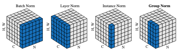
In summary:
- Group norm with one channel per group -> Instance norm
- Group norm with all channels in one group -> Layer norm
- Number of channels $C=1$: Layer norm = Instance norm
- Batch size $N=1$: Batch norm = Instance norm
Note that even the normalization is applied on groups, weights $\gamma_c,\beta_c$ are separate for each channel $c$. This makes the group normalization has the same learnable weights as the layer norm.
import keras
gnlayer = keras.layers.GroupNormalization(groups=4)
gnlayer.build([3,5,7,12])  # each group has 12/4=3 channels
print(gnlayer.weights)     # gamma, beta: both of shape (12,)
Weight normalization is to normalize weights instead of input/output tensors to a layer. Essentially this is a reparameterization of the weight. This is a trick to speed up convergence of SGD without any dependency to samples. A neural network operation is $y=\phi(\mathbf{w}\cdot\mathbf{x}+b)$ and weight normalization is to write
\[\mathbf{w} = \frac{g}{\Vert\mathbf{v}\Vert}\mathbf{v}\]in which $g$ is a scalar and $\mathbf{v}$ is a tensor with the same shape as $\mathbf{w}$. SGD and weight update is on $\mathbf{v}$ only while keeping $y=\phi(\mathbf{w}\cdot\mathbf{x}+b)$. This way, the scaled gradient (of $\mathbf{v}$, from $\mathbf{w}$) self-stablizes the norm.
Spectral Normalization was introduced to improve the training of GAN in which there is an issue of mode collapse. It is a phenomenon when the generative model’s output is homogeneous, failing to cover the full range of true data distribution, but only producing highly similar results. Recall that Lipschitz continuity is where
\[d_Y(f(x_1), f(x_2)) \le K d_X(x_1, x_2)\]for distance metrics $d_X,d_Y$ and $K$ the Lipschitz constant. Assume the neural network is a function $f$, it is to control the bi-Lipschitzness:
\[L_1\Vert x_1-x_2 \Vert_X \le \Vert f(x_1)-f(x_2)\Vert_F \le L_2\Vert x_1-x_2\Vert_X\]or to impose $\Vert\nabla f\Vert=1$. This is achieved by dividing the weight matrix by its largest singular value (a.k.a. the spectral norm of the matrix, hence the name).
RMS Norm is the late invention. Instead of normalization by mean and variance, it scales the input by its root mean square and typically not centering it. As a result, only the scaling parameter $\gamma$ is learnable and there is absence of the shift parameter $\beta$. This makes RMS norm simpler and faster.
Keras does not have a RMS norm implementation (yet). You need to write your own class:
import tensorflow as tf
from keras import backend as K

class RMSNorm(tf.keras.layers.Layer):
    def __init__(self, epsilon=1e-8, **kwargs):
        super(RMSNorm, self).__init__(**kwargs)
        self.epsilon = epsilon

    def build(self, input_shape):
        self.gamma = self.add_weight(name='gamma',
                                     shape=(input_shape[-1],),
                                     initializer='ones',
                                     trainable=True)
        super(RMSNorm, self).build(input_shape)

    def call(self, inputs):
        rms = K.sqrt(K.mean(K.square(inputs), axis=-1, keepdims=True))
        return inputs * self.gamma / (rms + self.epsilon)

    def get_config(self):
        config = super(RMSNorm, self).get_config()
        config.update({'epsilon': self.epsilon})
        return config
Note that in this implementation, the RMS is computed over the last axis of the input tensor x, i.e., over the channel dimension, matching the author’s reference code at https://github.com/bzhangGo/rmsnorm. In equations:
References
- Sergey Ioffe and Christian Szegedy (2015) Batch normalization: Accelerating deep network training by reducing internal covariate shift. arXiv:1502.03167.
- Jimmy Lei Ba and Jamie Ryan Kiros and Geoffrey E. Hinton (2016) Layer normalization. arXiv:1607.06450.
- Dmitry Ulyanov and Andrea Vedaldi and Victor Lempitsky (2016). Instance normalization: The missing ingredient for fast stylization. arXiv:1607.08022.
- Yuxin Wu and Kaiming He (2018). Group normalization. In Proceedings of the European conference on computer vision (ECCV) (pp. 3-19). arXiv:1803.08494.
- Tim Salimans and Diederik P. Kingma (2016). Weight normalization: A simple reparameterization to accelerate training of deep neural networks. In Advances in neural information processing systems (pp. 901-909). arXiv:1603.07868.
- Takeru Miyato and Toshiki Kataoka and Masanori Koyama and Yuichi Yoshida (2018) Spectral normalization for generative adversarial networks. In Proc. ICLR arXiv1802.05957.
- Biao Zhang and Rico Sennrich (2019) Root Mean Square Layer Normalization. In Proc. NeurIPS. arXiv:1910.07467.
- Jingjing Xu, Xu Sun, Zhiyuan Zhang, Guangxiang Zhao, and Junyang Lin (2019) Understanding and Improving Layer Normalization. In Proc. NeurIPS arXiv:1911.07013