This is a paper from Apple, targeted to create a backbone network that is fast enough to use on mobile devices. One characteristic of the network is that is decoupled the train-time and inference-time architecture. The trained model will be reparameterized for inference to make it more efficient.
The efficiency of an image classification model should be measured by latency. This is hardware dependent, so some may use number of FLOPs or the number of parameters as a proxy. The paper argues that these are incorrect. Sharing parameters can reduce the model size but increase FLOPs. Some parameter-free operations such as skip-connections and branching can incur memory access overhead. The paper said there are many models with high parameter count with lower latency. Also, convolutional models with similar parameter count is faster than transformer counterparts.
The paper proposed a network that, in the inference architecture, is simple feed-forward structure without any branches or skip-connections. Several techniques are used to lower the latency:
- Use only ReLU instead of other activations such as SE-ReLU or DynamicReLU because they incur synchronization overhead
- Multibranch architecture incurs memory access cost as activation from each branch needs to be stored
- Global pooling forces synchronization, also increases latency
The MobileOne network builds on MobileOne blocks. The blocks are over-parameterized to improve accuracy. The basic block is a $3\times 3$ depthwise convolution followed by a $1\times 1$ pointwise convolution. Then added a skip connection with batchnorm. As in the official code (simplified):
class MobileOneBlock(nn.Module):
    def __init__(self, in_channels: int, out_channels: int, kernel_size: int, ...):
        ...
        self.se = SEBlock(out_channels)
        self.activation = nn.ReLU()

        self.rbr_skip = nn.BatchNorm2d(num_features=in_channels)
        self.rbr_conv = nn.ModuleList([
            self._conv_bn(kernel_size=kernel_size, padding=padding)
            for _ in range(self.num_conv_branches)
        ])
        self.rbr_scale = self._conv_bn(kernel_size=1, padding=0)

    def forward(self, x: torch.Tensor) -> torch.Tensor:
        identity_out = self.rbr_skip(x)
        scale_out = self.rbr_scale(x)
        out = scale_out + identity_out
        for ix in range(self.num_conv_branches):
            out += self.rbr_conv[ix](x)
        return self.activation(self.se(out))

    def _conv_bn(self, kernel_size: int, padding: int):
        mod_list = nn.Sequential()
        mod_list.add_module("conv", nn.Conv2d(in_channels=self.in_channels,
                                              out_channels=self.out_channels,
                                              kernel_size=kernel_size,
                                              groups=self.groups,
                                              ...)
        mod_list.add_module("bn", nn.BatchNorm2d(num_features=self.out_channels)
        return mod_list
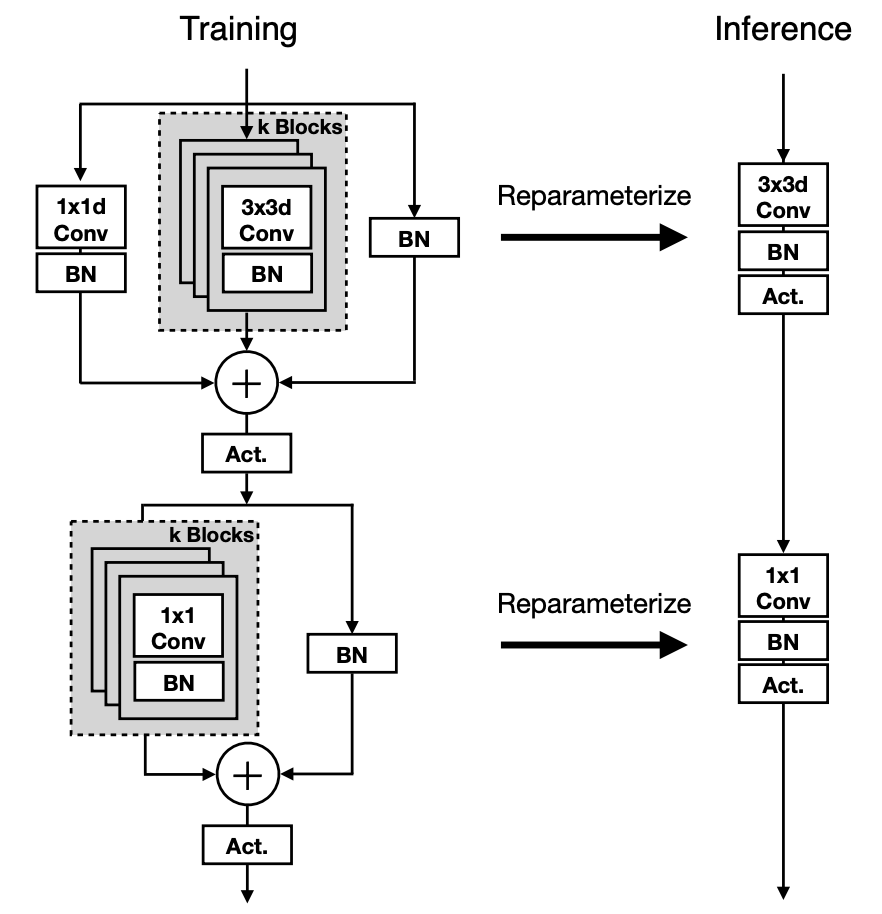
The rbr_skip branch is just a batchnorm, corresponds to the right branch of the first training block in the figure. The rbr_scale branch is a pointwise conv ($1\times 1$ conv) with a batchnorm, corresponds to the left branch. The rbr_conv is a list of $k$ $3\times 3$ conv bn. The conv will be depthwise if self.groups == self.in_channels. The output of one block is the sum of all branches. The over-parameterization factor $k$ varied from 1 to 5.
At inference, all these branches are reparameterized to a single conv with batchnorm fused (the figure is inaccurate).
The full network is a stack of 5 stages, then an average pooling layer and a linear layer as the classifier head. In stage 0, it is just a MobileOne block with $3\times 3$ kernel. Then in stages 1 to 4, each stage is a stack of MobileOne blocks with each $3\times 3$ depthwise conv followed by a MobileOne block with $1\times 1$ conv. The number of block pairs in each stage are [2, 8, 10, 1], meaning there are 4, 16, 20, and 2 MobileOne blocks in stages 1 to 4, with the $3\times 3$ and $1\times 1$ interleaved.
The number of channels in each stage are [64, 128, 256, 512], each multiplied by a width multiplier $w$. In variant “s1”, the width multipliers are [1.5, 1.5, 2.0, 2.5], meaning the number of channels are [96, 192, 512, 1280]. The number of channels in the last stage is the size of the output of the final pooling layer.
Squeeze and excitation network
The MobileOne network uses the “Squeeze and Excite” block in the variant “s4”. This is an optional module. If used, it is applied on the output of each MobileOne block right before the activation function.
The SE block originated from the following paper:
@misc{hu2017squeeze,
  title={Squeeze-and-excitation networks},
  authors={Jie Hu and Li Shen and Samuel Albanie and Gang Sun and Enhua Wu},
  year={2017},
  howpublished={arXiv preprint arXiv:1709.01507},
  url={https://github.com/hujie-frank/SENet},
}
A convolutional operator transfer an image into feature map:
\[\mathbf{F} = \mathbb{R}^{H'\times W'\times C'} \mapsto \mathbb{R}^{H \times W \times C}\]It is applied spatially and across channels. In equation, with the bias term omitted for brevity, the output feature map $\mathbf{u}_c$ is sum through all input channels:
\[\begin{aligned} \mathbf{V} &= [\mathbf{v}_1, \mathbf{v}_2, \cdots, \mathbf{v}_C] & \text{(learned filter kernels for each channel)} \\ \mathbf{U} &= [\mathbf{u}_1, \mathbf{u}_2, \cdots, \mathbf{u}_C] & \text{(feature maps)} \\ \mathbf{u}_c &= \mathbf{v}_c * \mathbf{X} = \sum_{s=1}^{C'} \mathbf{v}_c^s * \mathbf{x}^s & \text{(convolution for one output channel)} \\ \end{aligned}\]It fused spatial and channel-wise information in a local receptive field. No guarantee that the channel-wise information is useful. SE block is to scale the feature map with a channel-wise scaling factor to emphasize the useful channels.
SE block is a squeeze followed by an excitation. It recalibrates the channel importance to improve the representational power. It first squeeze, which is simply a global average pooling:
\[z_c = \mathbf{F}_{sq}(\mathbf{u}_c) = \frac{1}{H \times W} \sum_{i=1}^{H} \sum_{j=1}^{W} u_c(i,j)\]The output $z_c \in \mathbb{R}^C$ is the statistics of each channel, averaged over all elements $u_c(i,j)$ in channel $c$.
Then the excitation is to capture the channel-wise dependencies. It use one FC layer with ReLU activation to reduce the dimensionality of the channel statistics ($\mathbf{y}_1 = \delta(\mathbf{W}_1 \mathbf{z})$), then a second FC layer with sigmoid activation to restore the dimensionality ($\mathbf{s} = \sigma(\mathbf{W}_2 \mathbf{y}_1)$). This is the computed channel-wise scaling factor to apply to the original feature map. In formula:
\[\begin{aligned} \mathbf{s} &= \mathbf{F}_{ex}(\mathbf{z}, \mathbf{W})= \sigma(\mathbf{W}_2\delta(\mathbf{W}_1 \mathbf{z})) && \text{(scaling factor)} \\ \tilde{\mathbf{x}}_c &= \mathbf{F}_{scale}(\mathbf{u}_c, s_c) = s_c \mathbf{u}_c && \text{(channel-wise scaling with $s_c$)} \\ \mathbf{W}_1 &\in \mathbb{R}^{\frac{C}{r} \times C} && \text{(reduction FC layer)} \\ \mathbf{W}_2 &\in \mathbb{R}^{C \times \frac{C}{r}} && \text{(restoration FC layer)} \\ \mathbf{z} &\in \mathbb{R}^C && \text{(squeeze output)} \\ \mathbf{s} &\in \mathbb{R}^C && \text{(channel scaling factor)} \\ \tilde{\mathbf{X}} &= [\tilde{\mathbf{x}}_1, \tilde{\mathbf{x}}_2, \cdots, \tilde{\mathbf{x}}_C] \in \mathbb{R}^{H \times W \times C} && \text{(scaled feature map)} \end{aligned}\]The squeeze-and-excitation paper gives an example of how this can be used in standard architectures, such as VGGNet or ResNet. For example, the Inception network is built with stacks of inception modules where each can be represented as $\tilde{\mathbf{X}} = \mathbf{F}_{tr}(\mathbf{X})$. Then with the SE block, it is modified to:
\[\begin{aligned} \mathbf{X}' &= \mathbf{F}_{tr}(\mathbf{X}) \in \mathbb{R}^{H \times W \times C} && \text{(original inception module)} \\ \mathbf{z} &= \mathbf{F}_{sq}(\mathbf{X}') \in \mathbb{R}^C && \text{(squeeze by global pooling)} \\ \mathbf{y}_1 &= \delta(\mathbf{W}_1 \mathbf{z}) \in \mathbb{R}^{\frac{C}{r}} && \text{(reduce dimensionality)} \\ \mathbf{s} &= \sigma(\mathbf{W}_2 \mathbf{y}_1) \in \mathbb{R}^C && \text{(restore dimensionality)} \\ &= \mathbf{F}_{ex}(\mathbf{z}, \mathbf{W}) \\ \tilde{\mathbf{X}} &= \mathbf{F}_{scale}(\mathbf{X}', \mathbf{s}) \in \mathbb{R}^{H \times W \times C} && \text{(channel-wise scaling)} \\ &= \mathbf{s} \odot \mathbf{X}' \end{aligned}\]and in ResNet, there is skip connection. So the output is similar to the above but the scaling is applied to the residual only:
\[\tilde{\mathbf{X}} = \mathbf{X} + \mathbf{F}_{scale}(\mathbf{X}', \mathbf{s}) \in \mathbb{R}^{H \times W \times C}\]It is found to improve on CNN at slight additional computational cost, surpassing on ILSVRC 2017 classification.
The implementation in the MobileOne code is:
class SEBlock(nn.Module):
    """Squeeze and Excite module."""
    def __init__(self, in_channels: int, rd_ratio: float = 0.0625):
        """ Construct a Squeeze and Excite Module.

        :param in_channels: Number of input channels.
        :param rd_ratio: Input channel reduction ratio.
        """
        super().__init__()
        self.reduce = nn.Conv2d(in_channels=in_channels,
                                out_channels=int(in_channels * rd_ratio),
                                kernel_size=1,
                                stride=1,
                                bias=True)
        self.expand = nn.Conv2d(in_channels=int(in_channels * rd_ratio),
                                out_channels=in_channels,
                                kernel_size=1,
                                stride=1,
                                bias=True)
    def forward(self, inputs: torch.Tensor) -> torch.Tensor:
        n, c, h, w = inputs.size()
        x = F.avg_pool2d(inputs, kernel_size=[h, w])  # average into one value per channel
        x = self.reduce(x)
        x = F.relu(x)
        x = self.expand(x)
        x = torch.sigmoid(x)
        x = x.view(-1, c, 1, 1)
        return inputs * x
Since it is just a channel-wise scaling, SE block is optional and not used in most of the MobileOne variants. If it is used, it is applied at the output of a MobileOne block where the feature map is dispatched.
High-level MobileOne architecture
MobileOne architrecture is a stack of 5 stages, excluding the classifier head. Each stage has a different number of channels in the feature maps. All stages are a stack of MobileOne blocks. The number of blocks in each stage varies.
In code, it is implemented as:
class MobileOne(nn.Module):
    ...
    def forward(self, x: torch.Tensor) -> torch.Tensor:
        """ Apply forward pass. """
        x = self.stage0(x)  # Sequential of MobileOne blocks
        x = self.stage1(x)
        x = self.stage2(x)
        x = self.stage3(x)
        x = self.stage4(x)
        x = self.gap(x)     # AdaptiveAvgPool2d
        x = x.view(x.size(0), -1)
        x = self.linear(x)  # logit for classification
        return x
The self.linear is the prediction head for classification. The self.gap is adaptive average pooling, which in this case is same as global average pooling per channel. Adaptive average pooling is a convenience that you specify only the output size, not the stride and kernel size (a.k.a. stencil size), and the network will automatically calculate them (paper: https://arxiv.org/pdf/1406.4729). In pseudocode:
stride: float = output / input
# kernel_size = stride
for i in range(len(output)):
  output[i] = mean(input[floor(i * stride): ceil((i+1) * stride)])
and as a PyTorch example:
m = nn.AdaptiveAvgPool2d(5)  # output size = 5
x = torch.randn(1, 1, 8)   # input size = 8
y = m(x)  # shape[-1] = 5
# mean as computed in (x[0],x[1]), (x[1],x[2],x[3]), (x[3],x[4]), (x[4],x[5],x[6]), (x[6],x[7])
Note that the adaptive average pooling will not change the number of channels.
Each stage in the MobileOne network is a number of interleaved depthwise and pointwise MobileOne blocks:
- if depthwise, there will be $C$ input channels, $C$ output channels, $3\times3$ kernel, padding 1, stride $S$, $C$ groups
- if pointwise, there will be $C$ output channels, $C’$ input channels, $1\times1$ kernel, padding 0, stride 1, 1 group; the subsequent block start with $C’$ input channels
Recall that the PyTorch Conv2D block has parameters in_channels, out_channels, kernel_size, stride, padding (an int, a tuple of int, or strings “valid” or “same”), dilation, groups (an int divides both the number of input and output channels, controlling how the input and output are connected), bias, padding_mode (“zeros”, “reflect”, “replicate”, or “circular”), device, dtype. It implements cross-correlation operation:
\(\text{out}(N_i, C_{\text{out}_j}) = \text{bias}(C_{\text{out}_j}) + \sum_{k=0}^{C_{\text{in}}-1} \text{weight}(C_{\text{out}_j}, k) \star \text{input}(N_i, k)\)
(See A guide to convolution arithmetic for deep learning and its GitHub).
All MobileOne block in each stage shared the fixed number of output channels $C’$. Only the first block in each stage may have $C\ne C’$. Officially, there are variants s0 to s4. They all shared the similar architecture with a different width multiplier $w$ that scaled the number of channels in each stage.
If SE block is used, it is applied on the last few blocks of each stage. The number of MobileOne blocks with SE blocks is a network configuration parameter in each stage.
Reparameterization
Reparameterization is to convert a trained model to a simpler form for faster inference. At the high level, it is the following function in the official code:
def reparameterize_model(model: torch.nn.Module) -> nn.Module:
    model = copy.deepcopy(model)
    for module in model.modules():
        if hasattr(module, 'reparameterize'):
            module.reparameterize()
    return model
The model architecture at the highest level does not change. But each MobileOneBlock class implemented a reparameterize method. The official implementation of MobileOneBlock has the following constructor:
class MobileOneBlock(nn.Module):
    def __init__(self, in_channels: int, out_channels: int, kernel_size: int,
                 stride: int = 1, padding: int = 0, dilation: int = 1,
                 groups: int = 1, inference_mode: bool = False,
                 use_se: bool = False, num_conv_branches: int = 1):
        super().__init__()
        self.inference_mode = inference_mode
        self.groups = groups
        self.stride = stride
        self.kernel_size = kernel_size
        self.in_channels = in_channels
        self.out_channels = out_channels
        self.num_conv_branches = num_conv_branches

        self.se = SEBlock(out_channels) if use_se else nn.Identity()
        self.activation = nn.ReLU()
        if inference_mode:
            self.reparam_conv = nn.Conv2d(in_channels=in_channels,
                                          out_channels=out_channels,
                                          kernel_size=kernel_size,
                                          stride=stride,
                                          padding=padding,
                                          dilation=dilation,
                                          groups=groups,
                                          bias=True)
        else:
            # Re-parameterizable skip connection
            self.rbr_skip = None
            if out_channels == in_channels and stride == 1:
                self.rbr_skip = nn.BatchNorm2d(num_features=in_channels)
            # Re-parameterizable conv branches
            self.rbr_conv = nn.ModuleList([
                self._conv_bn(kernel_size=kernel_size, padding=padding)
                for _ in range(self.num_conv_branches)
            ])
            # Re-parameterizable scale branch: 1x1 conv to reset the channel dimension
            self.rbr_scale = None
            if kernel_size > 1:
                self.rbr_scale = self._conv_bn(kernel_size=1, padding=0)

    def forward(self, x: torch.Tensor) -> torch.Tensor:
        if self.inference_mode:
            return self.activation(self.se(self.reparam_conv(x)))

        identity_out = 0
        if self.rbr_skip is not None:
            identity_out = self.rbr_skip(x)
        scale_out = 0
        if self.rbr_scale is not None:
            scale_out = self.rbr_scale(x)
        out = scale_out + identity_out
        for ix in range(self.num_conv_branches):
            out += self.rbr_conv[ix](x)
        return self.activation(self.se(out))
The inference_mode argument is False by default, creating the multi-branch block in the training model. In the training mode, Conv2D layers will have no bias since there is a BatchNorm layer following to provide the scale and shift. In inference mode, only the SE block, Conv2D, and ReLU activation are used. It is to return ReLU(SE(Conv(x))) where the SE part is optional, but the Conv2D layer has a bias term.
Reparameterization is to recreate the Conv2D block with specific weights then delete the training mode branches and set inference_mode to True.
Here is how the reparameterization works. Recall that batch norm performs, with running mean $\mu_c$ and var $\sigma_c^2$ and learned parameters $\gamma_c$ and $\beta_c$,
\[y_{nhwc} = \frac{\gamma_c}{\sqrt{\sigma_c^2 + \epsilon}} x_{nhwc} + \beta_c - \frac{\gamma_c\mu_c}{\sqrt{\sigma_c^2 + \epsilon}}\]The rbr_skip (the lone BatchNorm2d as “identity out”) will be a Conv2D layer with kernel of shape (C_in, C_in//groups, k, k), i.e., kernel size k, with zeros everywhere except the center (i.e., at location (:, :, k//2, k//2)). The value at the center is computed as:
std = sqrt(running_var + eps)
kernel = gamma / std   # multiplication at channel dimension
bias = beta - running_mean * gamma / std
where the running_mean and running_var are what batch norm computes and gamma and beta are the learned parameters in the BN layer. The eps=1e-5 is a constant in PyTorch.
All other branches in the training mode are Conv-BN blocks. Reparameterization is to create a Conv2D layer that copied the kernel from the original Conv2D layer as kernel, then with the parameters from the BN layer, compute:
std = sqrt(running_var + eps)
kernel = kernel * gamma / std   # multiplication at channel dimension
bias = beta - running_mean * gamma / std
and the kernel and bias are set to the new Conv2D layer. Note that rbr_scale is with kernel size 1. Its output will be zero-padded to match the block’s kernel size.
With all branches reparameterized, the kernel and bias of all branches are summed up to form the final reparameterized Conv2D layer. Below is the exact reparameterization code in the MobileOneBlock class:
class MobileOneBlock(nn.Module):
    ...
    def reparameterize(self):
        if self.inference_mode:
            return
        kernel, bias = self._get_kernel_bias()
        self.reparam_conv = nn.Conv2d(in_channels=self.rbr_conv[0].conv.in_channels,
                                      out_channels=self.rbr_conv[0].conv.out_channels,
                                      kernel_size=self.rbr_conv[0].conv.kernel_size,
                                      stride=self.rbr_conv[0].conv.stride,
                                      padding=self.rbr_conv[0].conv.padding,
                                      dilation=self.rbr_conv[0].conv.dilation,
                                      groups=self.rbr_conv[0].conv.groups,
                                      bias=True)
        self.reparam_conv.weight.data = kernel
        self.reparam_conv.bias.data = bias

        # Delete un-used branches
        for para in self.parameters():
            para.detach_()
        self.__delattr__('rbr_conv')
        self.__delattr__('rbr_scale')
        if hasattr(self, 'rbr_skip'):
            self.__delattr__('rbr_skip')

        self.inference_mode = True

    def _get_kernel_bias(self) -> Tuple[torch.Tensor, torch.Tensor]:
        # get weights and bias of scale branch
        kernel_scale = bias_scale = 0
        if self.rbr_scale is not None:
            kernel_scale, bias_scale = self._fuse_bn_tensor(self.rbr_scale)
            # Pad scale branch kernel to match conv branch kernel size.
            pad = self.kernel_size // 2
            kernel_scale = torch.nn.functional.pad(kernel_scale, [pad, pad, pad, pad])

        # get weights and bias of skip branch
        kernel_identity = bias_identity = 0
        if self.rbr_skip is not None:
            kernel_identity, bias_identity = self._fuse_bn_tensor(self.rbr_skip)

        # get weights and bias of conv branches
        kernel_conv = bias_conv = 0
        for ix in range(self.num_conv_branches):
            _kernel, _bias = self._fuse_bn_tensor(self.rbr_conv[ix])
            kernel_conv += _kernel
            bias_conv += _bias

        kernel_final = kernel_conv + kernel_scale + kernel_identity
        bias_final = bias_conv + bias_scale + bias_identity
        return kernel_final, bias_final

    def _fuse_bn_tensor(self, branch) -> Tuple[torch.Tensor, torch.Tensor]:
        if isinstance(branch, nn.Sequential):
            # for all normal ConvBN layers or the rbr_scale layer
            kernel = branch.conv.weight
            running_mean = branch.bn.running_mean
            running_var = branch.bn.running_var
            gamma = branch.bn.weight
            beta = branch.bn.bias
            eps = branch.bn.eps
        else:
            # only for rbr_skip, which is a lone BatchNorm2d layer
            assert isinstance(branch, nn.BatchNorm2d)
            input_dim = self.in_channels // self.groups
            kernel = torch.zeros((self.in_channels,
                                  input_dim,
                                  self.kernel_size,
                                  self.kernel_size),
                                  dtype=branch.weight.dtype,
                                  device=branch.weight.device)
            kernel[:, :, self.kernel_size // 2, self.kernel_size // 2] = 1
            running_mean = branch.running_mean
            running_var = branch.running_var
            gamma = branch.weight
            beta = branch.bias
            eps = branch.eps
        std = (running_var + eps).sqrt()
        t = (gamma / std).reshape(-1, 1, 1, 1)
        return kernel * t, beta - running_mean * gamma / std
Training of the MobileOne network
The paper reports that the model can achieve 75% top-1 accuracy on ImageNet. But the official code does not provide the training script. Here is what I did to train the model.
The model is trained with the following configuration:
- epochs: 300
- batch size: 256
- optimizer: SGD with momentum 0.9
- initial learning rate: 0.1, with cosine annealing
- weight decay: 1e-4, annealed with cosine schedule to 1e-5
- model EMA: 0.9999
- loss function: cross entropy with label smoothing 0.1
- augmentation: AutoAug with progressive strength for variant s2 to s4, or random resized crop and horizontal flip for variant s0 and s1
- training size:
- epochs 0-38: 160px
- epochs 39-113: 192px
- epochs 114-300: 224px
I used the timm library to train the model. I updated a bit the train.py to use the official mobileone code and make the training stop at a specific epoch and allow the checkpoint history to be reloaded. Other than that, the following are the training config YAML file:
aa: 'rand-inc1-n10-m1-mstd0.5'  # RandAugment
amp: false            # do not use mixed precision training
amp_dtype: bfloat16
amp_impl: native
aug_repeats: 0
aug_splits: 0
batch_size: 256       # single GPU
bce_loss: false
bce_pos_weight: null
bce_sum: false
bce_target_thresh: null
bn_eps: null
bn_momentum: null
channels_last: true   # use channel last
checkpoint_hist: 10
class_map: ''
clip_grad: null
clip_mode: norm
color_jitter: null    # disable color jitter
color_jitter_prob: null
cooldown_epochs: 0
crop_pct: null
cutmix: 0.0
cutmix_minmax: null
data: null
data_dir: '/mnt/dataset/ImageNet/' # imagenet training
#dataset: 'torch/imagenet'
dataset_download: true
dataset_trust_remote_code: true
decay_epochs: 90                   # irrelevant in Cosine Scheduler
decay_milestones: [90, 180, 270]
decay_rate: 0.1                    # irrelevant in Cosine Scheduler
device: cuda
device_modules: null
dist_bn: reduce                    # irrelevant, not using distributed training
drop: 0.0
drop_block: null
drop_connect: null
drop_path: null
epoch_repeats: 0.0
epochs: 295
eval_metric: top5          # default: top1 -> top5
experiment: 'my_mobileone_s1'
fast_norm: false
fuser: ''
gaussian_blur_prob: null
gp: null
grad_accum_steps: 1
grad_checkpointing: false  # custom model has no grad checkpointing
grayscale_prob: null
head_init_bias: null
head_init_scale: null
hflip: 0.5
img_size: null
in_chans: null
initial_checkpoint: ''
input_img_mode: null       # default RGB, PIL supports YCbCr, HSL, and others
input_key: null
input_size: [3, 224, 224]
interpolation: 'bilinear'  # default empty string = let model decide
jsd_loss: false
layer_decay: null
local_rank: 0
log_interval: 100          # more frequent print of LR and loss
log_wandb: false
lr: null                   # keep null, to compute based on lr_base and actual batch size
lr_base: 0.1               # keep default
lr_base_scale: ''
lr_base_size: 256
lr_cycle_decay: 0.5
lr_cycle_limit: 1
lr_cycle_mul: 1.0          # cycle 1 = no cycle
lr_k_decay: 1.0            # cosine: <1 for faster drop, >1 to stay high longer
lr_noise: null
lr_noise_pct: 0.67
lr_noise_std: 1.0
mean: [0.5, 0.5, 0.5]      # default [0.485, 0.456, 0.406)
min_lr: 1e-6               # 0 -> 1e-6
mixup: 0.0                 # no mixup augmentation
mixup_mode: batch
mixup_off_epoch: 0
mixup_prob: 1.0
mixup_switch_prob: 0.5
model: custom_mobileone    # e.g., timm/mobileone_s1.apple_in1k
model_dtype: null
model_ema: false           # not use EMA model
model_ema_decay: 0.9995    # 0.9998 -> momentum 5e-4
model_ema_force_cpu: false
model_ema_warmup: false
model_kwargs: {variant: s1}
momentum: 0.9
no_aug: false
no_ddp_bb: false
no_prefetcher: false
no_resume_opt: false
num_classes: 1000
opt: sgd  # <- keep default
opt_betas: null
opt_eps: null
opt_kwargs: {}
output: ''
patience_epochs: 10
pin_mem: false
pretrained: false
pretrained_path: null
ratio: [0.75, 1.3333333333333333]
recount: 1
recovery_interval: 0
remode: pixel
reprob: 0.0
resplit: false
resume: 'output/train/my_mobileone_s1/last.pth.tar'
save_images: false
scale: [0.08, 1.0]      # keep default, scaling in augmentation
sched: cosine
sched_on_updates: true  # default: false
seed: 42
smoothing: 0.1          # keep default, label smoothing
split_bn: false
start_epoch: null       # infer from checkpoint if resume path is set
#end_epoch: 114
std: [0.5, 0.5, 0.5]    # default [0.229, 0.224, 0.225)
sync_bn: false
synchronize_step: false
target_key: null
torchcompile: null      # expect a backend if used, e.g., inductor
torchcompile_mode: null
torchscript: false
train_crop_mode: rrc    # rkrr = resize keep ratio random crop, use in S2+
train_interpolation: 'bilinear'  # random -> bilinear
train_num_samples: null
train_split: train
tta: 0
use_multi_epochs_loader: true
val_num_samples: null
val_split: val
validation_batch_size: null
vflip: 0.0
wandb_project: null
wandb_resume_id: ''
wandb_tags: []
warmup_epochs: 5        # 5*10009 iterations due to sched_on_update=true
warmup_lr: 1e-5         # default 1e-5
warmup_prefix: true     # false -> true
weight_decay: 1.0e-04   # 2e-5 -> 4e-5
worker_seeding: all
workers: 16
Then you can run the training with timm by:
train.py -c train.yaml
and it takes a few days to finish from scratch.
Some explanation of the training:
Hugging Face hub already have a MobileOne model. If you use it, you can set the model to timm/mobileone_s1.apple_in1k and optionally, set pretrained to True to load the pretrained weights.
This training uses the ImageNet dataset, both the training set and validation set are used, and the checkpoint is saved for the best validation accuracy. The dataset should be stored in the location pointed by data_dir. In timm, the dataset can be loaded in multiple ways but reading from the file system is the fastest. Setting the dataset to a string torch/imagenet other than null will read the directory as a torchvision dataset, but I found it slower.
The ImageNet dataset is expected to have the following structure:
ImageNet/
  train/
    n01440764/
      n01440764_10026.JPEG
      ...
    ...
  val/
    n01440764/
      ILSVRC2012_val_00000001.JPEG
      ...
Essentially, the subdir under data_dir are the name of the “split”. Under each split, the subdirs are the class names. Make sure both splits share exact the same set of classes. Under each class subdir are images to be loaded using PIL.
The data loading and augmentation are slow but timm already optimized it using multiple processes. One way to boost the speed is to use Pillow-SIMD as the drop-in replacement of PIL. Also, scale the workers parameter for the platform to exhaust the CPU until I/O bandwidth is saturated.
The training is checkpointed. For the first step, you should comment out the resume line in the YAML file since there’s nothing to resume. At end of each step, you can update the parameters end_epoch, and input_size but keep the rest. Note that the model is trained in channel-last format but the input_size should always be specified in channel-first format.
I override the image normalization mean and std to an easy value of 0.5 and 0.5. This is applied when the image is loaded and the pixel values are already scaled to be between 0 and 1. These parameters will make the image pixel values to be between -1 and 1.
Augmentation is using RandAugment with configuration string “rand-inc1-n10-m1-mstd0.5”. See the timm documentation and in particular, the RandAugment part, this means number of operations is 10, the magnitude is 1, and the standard deviation of the magnitude is 0.5 with the augmentation increase in severity with magnitude. Not sure if it is the best, but using RandAugment is better than specifying augmentation in other ways. Therefore, the color jitter, blur, cutmix and mixup are all disabled. Random resized crop is used and it is applied before RandAugment.
The training is in 300 epochs in total. Each epoch will scan through the 1.28M training images from ImageNet dataset once. There are 5 warm up epochs, so the epoch count in the YAML file is 295. Cosine scheduler is used according to the paper, but the learning rate update is per step, not per epoch. EMA is recommended by the paper, but I think the momentum of 5e-4 is too small that the half-life does not match the number of epochs trained. Hence, I disabled it.
I set up three YAML files for the three steps in training with different image sizes (this is a purely conv model, hence the image size does not matter). A decent GPU can achieve 2000 images per second in training. That amounts to around 54 hours of training time from scratch.
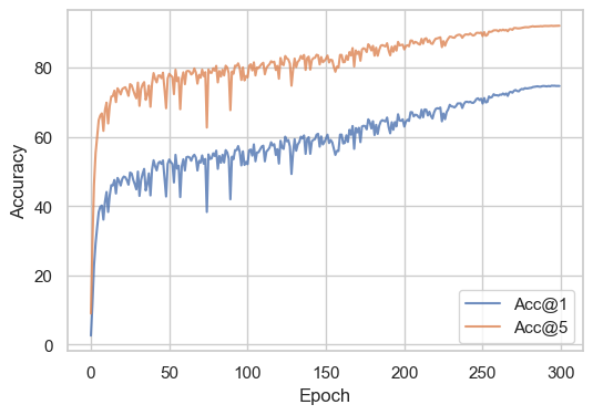
This training recipe achieved 75% top-1 accuracy on ImageNet. The loss curve is shown below:
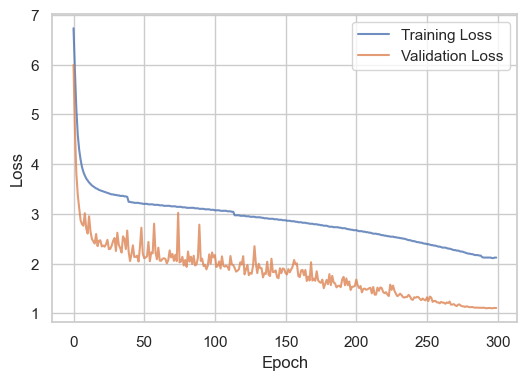
and the accuracy curve is shown below:
Bibliographic data
@inproceedings{
   title = "MobileOne: An Improved One millisecond Mobile Backbone",
   author = "Pavan Kumar Anasosalu Vasu and James Gabriel and Jeff Zhu and Oncel Tuzel and Anurag Ranjan",
   booktitle = "Proc. CVPR",
   year = "2023",
   arxiv = "2206.0404",
   github = "https://github.com/apple/ml-mobileone",
}