The Lipschutz continuity definition inspired me on how to distort a curve to “smooth out” outliers. Smoothing out means that we want to retain most characteristics of a curve if it falls within proximity of the mean (for whatever definition of proximity and mean) and for the part that the curve is distorted, it should not depends on explicit parameters. Thus, for example, cap the curve \(y=f(x)\) into \(y=\min(f(x),M)\) is less favorible because the cap \(M\) has to be dependent to \(f(x)\) to be useful.
Recall that Lipschutz continuity means:
\[||f(x_1)-f(x_2)||_2 \le k ||x_1-x_2||_2\]Roughly speaking, the slope of \(f(x)\) is bounded (by \(k\)), for slope is defined as if \((x,f(x))\) is connected. Now consider a simplified function to make the problem tractable, namely, \(f(x)\) is monotonically increasing and defined only on \(x\in X=[0,1]\). Then the outlier is either at the proximity of 0 or 1, and the derivative \(f'(x)\ge 0\) due to monotonicity.
If we define a modified derivative, \(g(x) = \min(f'(x), k)\) for some \(k>0\), then we have an approximate of \(f(x)\) as
\[\hat{f}(x) = \int_{x_0}^x g(x) dx + f(x_0) \quad \exists x_0 \in X\]Consider the case \(x_0\) is roughly at the middle portion \(X'\) of \(X=[0,1]\) and \(k\) is defined as
\[k = \alpha \max_{x\in X'} f'(x) \quad \alpha\ge 1, X'\subset X\]Then \(\hat{f}(x)\) will be exactly the same as \(f(x)\) for \(x\in X'\), and it will be distorted from \(f(x)\) at \(x\notin X'\) iff \(f'(x)\) too large (gauged by \(\alpha\)).
Let’s look at an example (code in Julia):
using PyPlot

function outlier_distort(vector, xmin, xmax)
    N = length(vector)
    imin = round(Int, (xmin * (N-1)) + 1)
    imax = round(Int, (xmax * (N-1)))
    delta = vector[2:end] - vector[1:end-1]
    maxdelta = maximum(delta[imin:imax]) # max element in delta[imin:imax]
    delta = min.(delta, fill(maxdelta, size(delta))) # elementwise cap delta to maxdelta
    newvector = foldl( (v,x)->push!(v,v[end]+x), [vector[1]], delta)
    offset = newvector[round(Int,N/2)] - vector[round(Int,N/2)]
    return newvector .- offset
end

value = [30.67, 31.88, 31.99, 32.11, 32.19, 32.56, 32.61, 32.89, 32.90, 32.91,
         32.94, 33.02, 33.08, 33.16, 33.41, 33.74, 33.77, 33.92, 33.96, 34.07,
         34.12, 34.14, 34.18, 34.18, 34.25, 34.33, 34.33, 34.33, 34.36, 34.36,
         34.38, 34.51, 34.55, 34.57, 34.59, 34.59, 34.62, 34.68, 34.68, 34.70,
         34.72, 34.74, 34.79, 34.86, 34.86, 34.89, 34.91, 34.92, 34.96, 34.97,
         34.98, 35.00, 35.00, 35.00, 35.01, 35.03, 35.03, 35.03, 35.03, 35.05,
         35.05, 35.06, 35.09, 35.09, 35.09, 35.12, 35.13, 35.14, 35.19, 35.19,
         35.24, 35.25, 35.25, 35.27, 35.27, 35.29, 35.29, 35.35, 35.36, 35.38,
         35.40, 35.41, 35.43, 35.50, 35.50, 35.56, 35.60, 35.60, 35.63, 35.66,
         35.66, 35.68, 35.68, 35.69, 35.71, 35.71, 35.71, 35.74, 35.76, 35.76,
         35.77, 35.78, 35.78, 35.80, 35.80, 35.81, 35.81, 35.81, 35.82, 35.83,
         35.85, 35.87, 35.87, 35.88, 35.89, 35.89, 35.89, 35.89, 35.90, 35.91,
         35.93, 35.94, 35.94, 35.94, 35.94, 35.97, 35.97, 35.98, 36.00, 36.00,
         36.01, 36.01, 36.01, 36.02, 36.03, 36.03, 36.03, 36.03, 36.04, 36.04,
         36.07, 36.11, 36.11, 36.11, 36.12, 36.12, 36.16, 36.17, 36.17, 36.19,
         36.19, 36.20, 36.21, 36.21, 36.24, 36.24, 36.25, 36.26, 36.39, 36.39,
         36.39, 36.39, 36.44, 36.46, 36.58, 36.69, 36.90, 37.02, 37.08, 37.11,
         37.15, 37.16, 37.18, 37.37, 37.69, 37.71, 37.71, 37.74, 37.87, 37.92,
         37.97, 37.97, 38.02, 38.02, 38.05, 38.15, 38.22, 38.22, 38.25, 38.36,
         38.36, 38.38, 38.47, 38.55, 38.57, 38.63, 38.65, 38.65, 38.73, 38.76,
         38.76, 38.80, 38.80, 38.84, 38.85, 38.85, 38.91, 39.07, 39.09, 39.12,
         39.15, 39.27, 39.27, 39.32, 39.34, 39.42, 39.43, 39.46, 39.48, 39.50,
         39.57, 39.57, 39.59, 39.67, 39.70, 39.83, 39.87, 39.87, 39.88, 39.91,
         39.97, 40.00, 40.00, 40.05, 40.06, 40.06, 40.08, 40.11, 40.13, 40.16,
         40.23, 40.27, 40.30, 40.35, 40.35, 40.40, 40.41, 40.58, 40.58, 40.63,
         40.67, 40.68, 40.71, 40.71, 40.71, 40.83, 40.86, 40.87, 40.87, 40.92,
         41.01, 41.01, 41.03, 41.07, 41.12, 41.12, 41.23, 41.25, 41.25, 41.27,
         41.29, 41.33, 41.33, 41.34, 41.42, 41.47, 41.54, 41.58, 41.59, 41.65,
         41.65, 41.75, 41.85, 41.85, 41.85, 41.85, 41.88, 42.01, 42.32, 42.57,
         42.57, 42.61, 42.66, 42.66, 42.78, 42.78, 42.89, 42.93, 42.93, 43.05,
         43.21, 43.47, 43.60, 43.87, 44.06, 44.35, 45.04, 45.04, 45.09, 45.09,
         45.45, 46.02, 46.02, 46.52, 46.90, 46.90, 46.90, 46.90, 47.69, 50.52,
         55.76, 98.97, 99.07, 99.25, 99.28, 99.33, 99.40, 99.40, 99.42, 99.43,
         99.44, 99.44, 99.46, 99.47, 99.50, 99.55, 99.60, 99.79, 99.84]
N = max(size(value)...)
x = collect(1:N) ./ N
distorted = outlier_distort(value, 0.2, 0.8)
plot(x,value,x,distorted)
The function outlier_distort expects input of monotonically increasing
values, and finds \(k\) from the 20% to 80%-ile, with \(\alpha=1\). The plot of the
above code:
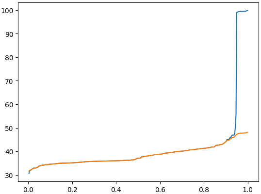
The orange line is the distorted curve \(y=\hat{f}(x)\) and the blue curve is \(y=f(x)\). We can notice that at above 0.95, that bit of flat curve looks alike in both colors albeit at different altitude. And the part that quickly ramps up in the blue curve is moderated in the orange curve such that it is less disruptive. A larger jump would be allowed if \(\alpha\) is larger.
The code above is suitable for \(f(x)\) a percentile function. For general \(f(x)\), we can use similar technique with a “translate” function that converts any value \(f(x)\) into \(\hat{f}(x)\). Such as the following:
function interpolate(invector, outvector, val)
r = searchsorted(invector, val)
lbound = invector[r.start]
ubound = invector[r.stop]
if lbound == ubound
return outvector[r.start]
else
ratio = (val-lbound)/(ubound-lbound)
return outvector[r.start] * ratio + outvector[r.stop] * (1-ratio)
end
end
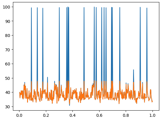
perm = shuffle(value)
distortedperm = [interpolate(value, distorted, v) for v=perm]
plot(x,perm,x,distortedperm)
Plot: