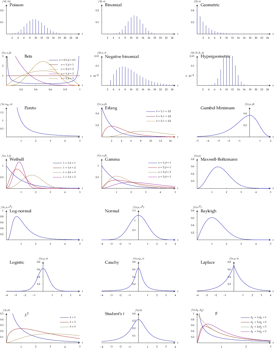
This is a summary of common probability distributions in engineering and statistics. This chart has the plots of the pdf or pmf (LaTeX source):

discrete distributions

binomial distribution

A big urn with balls in either white or black color. Drawing a white ball from urn has probability \(x\) (i.e., black ball has probability \(1-x\)). If we draw \(n\) balls from urn with replacement, the probability of getting \(k\) white balls:

\[f(k; n, x) = \binom{n}{k} x^k (1-x)^{n-k}\]

Poisson distribution

Balls are added to the urn at rate of \(\lambda\) per unit time, under exponential distribution. The probability of having \(k\) balls added to the urn within time \(t\):

\[f(k; \lambda t) = \frac{(\lambda t)^k e^{-\lambda t}}{k!}\]

geometric distribution

The probability of have to draw \(k\) balls to see the first white ball being drawn:

\[f(k; x) = (1-x)^{k-1} x\]

negative binomial distribution

same as the distribution of the sum of \(r\) iid geometric random variable
negative binomial approximates Poisson with \(\lambda = r(1-x)\) with large \(r\) and \(x\approx 1\)
Drawing balls from the urn. If we have to draw \(k\) balls to see the \(r\)-th white ball (we have drawn \(r\) white balls and \(k-r\) black balls). The probability of \(k\):

\[f(k; r, x) = \binom{k-1}{k-r} x^r (1-x)^{k-r}\]

hypergeometric distribution

A urn with \(N\) balls (finite) and \(K\) balls amongst are white. Draw, without replacement, \(n\) balls from the urn to get \(k\) white balls:

\[f(k; N, K, n) = \frac{\binom{K}{k}\binom{N-K}{n-k}}{\binom{N}{n}}\]

continuous distributions

uniform distribution

extreme of flattened distribution
with upper and lower bounds

triangular distribution

with upper and lower bounds

normal distribution

strong tendency for data at central value; symmetric, equally likely for positive and negative deviations from its central value
frequency of deviations falls off rapidly as we move further away from central value

\[f(x; \mu, \sigma^2) = \frac{1}{\sqrt{2\pi\sigma^2}}\exp(-\frac{(x-\mu)^2}{2\sigma^2})\]

\[X_1 \sim N(\mu_1, \sigma^2_1); X_2 \sim N(\mu_2, \sigma^2_2) \to X_1+X_2 \sim N(\mu_1+\mu_2, \sigma_1^2+\sigma_2^2)\]
approximation to Poisson distribution: if \(\lambda\) is large, Poisson distribution approximates normal with \(\mu=\sigma^2=\lambda\)
approximation to binomial distribution: if \(n\) is large and \(x\approx \frac{1}{2}\), binomial distribution approximates normal with \(\mu=nx\) and \(\sigma^2=nx(1-x)\)
approximation to beta distribution: if \(\alpha\) and \(\beta\) are large, beta distribution approximates normal with \(\mu=\frac{\alpha}{\alpha+\beta}\) and \(\sigma^2=\frac{\alpha\beta}{(\alpha+\beta)^2(\alpha+\beta+1)}\)

Laplace distribution

absolute difference from mean compared to squared difference in normal distribution
longer (fatter) tails, higher kurtosis (flattened peak)
pdf:

\[f(x; \mu, s) = \frac{1}{2s}\exp(-\frac{|x-\mu|}{s})\]

logistic distribution

symmetric, with longer tails and higher kurtosis than normal distribution
logistic distribution has finite mean \(\mu\) and variance defined
\[X\sim U(0,1) \to \mu+s[\log(X)-\log(1-X)] \sim \textrm{Logistic}(\mu,s)\]
\[X\sim \textrm{Exp}(1) \to \mu+s\log(e^X-1) \sim \textrm{Logistic}(\mu,s)\]
logistic pdf:

\[f(x; \mu, s) = \frac{e^{-(x-\mu)/s}}{s\left(1+e^{-(x-\mu)/s}\right)^2}\]

Cauchy distribution

symmetric, with longer tails and higher kurtosis than normal distribution
Cauchy distribution has mean and variance undefined, but mean & mode at \(\mu\)
\[X,Y\sim N(\mu,\sigma^2) \to X/Y \sim \textrm{Cauchy}(\mu,\sigma^2)\]
Cauchy pdf:

\[f(x; x_0, \gamma) = \frac{1}{\pi\gamma\left[1+\left(\frac{x-x_0}{\gamma}\right)^2\right]}\]

lognormal distribution

\(\log(X)\sim N(\mu,\sigma^2)\), positively skewed
parameterised by shape (\(\sigma\)), scale (\(\mu\), or median), shift (\(\theta\))
\(\mu=0, \theta=1\) is standard lognormal distribution
as \(\sigma\) rises, the peak shifts to left and skewness increases

\[f(x; \mu, \sigma^2) = \frac{1}{\sqrt{2\pi x^2\sigma^2}}\exp(-\frac{(\log x-\mu)^2}{2\sigma^2})\]

sum of two lognormal random variable is a lognormal random variable with \(\mu=\mu_1+\mu_2\) and \(\sigma^2=\sigma_1^2+\sigma_2^2\)

Pareto distribution

power law probability distribution
continuous counterpart of Zipf’s law
positively skewed, no negative tail, peak at \(x=0\)

\[f(x; x_m, \alpha) = \frac{\alpha x_m^{\alpha}}{x^{\alpha+1}}\]

gamma distribution

support for \(x\in(0,\infty)\), positive skewness (lean left)
decreasing \(\alpha\) will push distribution towards the left; at low \(\alpha\), left tail will disappear and distribution will resemble exponential
models the time to the \(\alpha\)-th Poisson arrival with arrival rate \(\beta\)
gamma pdf (\(\alpha=1\) becomes exponential pdf with rate \(\beta\)):

\[f(x; \alpha, \beta) = \frac{\beta^{\alpha}}{\Gamma(\alpha)} x^{\alpha-1}e^{-\beta x}\]

Weibull distribution

support for \(x\in(0,\infty)\), positive skewness (lean left)
decreasing \(k\) will push distribution towards the left; at low \(k\), left tail will disappear and distribution will resemble exponential
If \(W\sim\textrm{Weibull}(k,\lambda)\), then \(X=W^k \sim \textrm{Exp}(1/\lambda^k)\)
Weibull pdf (\(k=1\) becomes exponential pdf with rate \(1/\lambda\)):

\[f(x; k, \lambda) = \frac{k}{\lambda}\left(\frac{x}{\lambda}\right)^{k-1}e^{-(x/\lambda)^k}\]

Erlang distribution

\[X_i\sim\textrm{Exp}(\lambda) \to \sum_{i=1}^k X_i \sim \textrm{Erlang}(k, \lambda)\]
arise from teletraffic engineering: time to \(k\)-th call

\[f(x; k,\lambda) = \frac{\lambda^k x^{k-1} e^{-\lambda x}}{(k-1)!}\]

beta distribution

support for \(x\in(0,1)\)
allows negative skewness
two shape parameters \(p\) and \(q\), and lower- and upper-bounds on data (\(a\) and \(b\))

\[f(x; \alpha, \beta) = \left(\frac{\Gamma(\alpha)\Gamma(\beta)}{\Gamma(\alpha+\beta)}\right)^{-1} x^{\alpha-1}(1-x)^{\beta-1}\]

extreme value distribution (i.e. Gumbel minimum distribution)

negatively skewed
Gumbel maximum distribution, \(f(-x;-\mu,\beta)\), is positively skewed
Limiting distribution of the max/min value of \(n\to\infty\) iid samples from \(\textrm{Exp}(\lambda)\) with \(\lambda = 1/\beta\)
standard cdf: \(F(x)=1-\exp(-e^x)\)

\[f(x; \mu, \beta) = \frac{1}{\beta}e^{(\mu-x)/\beta}e^{-e^{(\mu-x)/\beta}}\]

Rayleigh distribution

positively skewed
modelling the \(L^2\)-norm of two iid normal distribution with zero mean (e.g., orthogonal components of a 2D vector)

\[f(x; \sigma) = \frac{x}{\sigma^2} \exp(-\frac{x^2}{2\sigma^2})\]

Maxwell-Boltzmann distribution

positively skewed
3D counterpart of Rayleigh distribution
arise from thermodynamic: probability of a particle in speed \(v\) if temperature is \(T\)

\[\begin{align} f(v; \sqrt{kT/m}) &= \left(\frac{m}{2\pi kT} \right)^{3/2} 4\pi v^2 \exp(-\frac{mv^2}{2kT}) \\ f(x; a) &= \sqrt{\frac{2}{\pi}}\frac{x^2 e^{-x^2/(2a^2)}}{a^3} \end{align}\]

Chi-squared distribution

distribution of the sum of the square of \(k\ge 1\) i.i.d. standard normal random variables
mean \(k\), variance \(2k\)
PDF with \(k\) degrees of freedom:

\[f(x; k) = \frac{x^{k/2-1} e^{-x/2}}{2^{k/2}\Gamma(k/2)}\]

F-distribution

Distribution of a random variable defined as the ratio of two independent \(\chi^2\)-distributed random variables, with degrees of freedom \(d_1\) and \(d_2\) respectively
Commonly used in ANOVA
PDF, with degrees of freedom \(d_1\) and \(d_2\), involves beta function \(B(\alpha,\beta)\):

\[\begin{align} f(x; d_1, d_2) &= \left[x B(\frac{d_1}{2},\frac{d_2}{2})\right]^{-1} \sqrt{\frac{(d_1 x)^{d_1} d_2^{d_2}}{(d_1 x+d_2)^{d_1+d_2}}} \\ \textrm{and if}\qquad z_1 &\sim \chi^2(d_1) \\ z_2 &\sim \chi^2(d_2) \\ \textrm{then}\qquad x = \frac{z_1/d_1}{z_2/d_2} &\sim f(x, d_1, d_2) \end{align}\]

Student’s t distribution

Distribution of normalized sample mean of \(n=k+1\) observations from a normal distribution, \(\frac{\bar{X}-\mu}{S/\sqrt{n}}\)
Equivalently, this is the distribution of \(\frac{x}{\sqrt{y/r}}\) for \(x\) is standard normal and \(y\) is chi-square with \(r\) degrees of freedom
t distribution with \(n=1\) is Cauchy distribution
PDF with degree of freedom \(k\):

\[f(x, k) = \frac{\Gamma(\frac{k+1}{2})}{\sqrt{k\pi}\Gamma(k/2)} \left(1+\frac{x^2}{k}\right)^{-(k+1)/2}\]

test of fit for distributions

Kolmogorov-Smirnov test (K-S test, on cumulative distribution function \(F(x)\))

\[D_n = \sup_x | F_n(x) - F(x) |\]

if sample comes from distribution, \(D_n\) converges to 0 a.s. as number of samples \(n\) goes to infinity

Shapiro-Wilk test

\[W = \frac{\sum_{i=1}^n a_i x_i}{\sum_{i=1}^n (x_i - \bar{x})^2}\]

test of normality in frequentist statistics (i.e. for \(x_i\) in normal distribution)
\(\bar{x} = \frac{1}{n}(x_1 + \cdots + x_n)\) is the sample mean
\((a_1,\cdots,a_n) = m^T V^{-1} (m^T V^{-1}V^{-1} m)^{-1/2}\) where \(m\) is vector of expected values of the order statistics from normal distribution and \(V\) the covariance matrix of those order statistics

Anderson-Darling test

\[A^2 = n \int_{-\infty}^{\infty} \frac{(F_n(x)-F(x))^2}{F(x)(1-F(x))} dF(x)\]

test whether a sample comes from a specified distribution
\(A^2\) is weighted distance between \(F_n(x)\) and \(F(x)\), with more weight on tails of the distribution

Pearson’s \(\chi^2\) test

\[\chi^2 = \sum_{i=1}^n \frac{(O_i - E_i)^2}{E_i}\]

test for categories fit a distribution: checking observed frequency \(O_i\) against expected frequency \(E_i\) according to distribution for each of \(n\) categories
degree of freedom: \(n\) minus number of parameters of the fitted distribution

Reference

Lawrence M. Leemis and Jacquelyn T. McQuestion. Univariate Distribution Relationships, Am Stat, 62(1) pp.45–53, 2008, DOI: 10.1198/000313008X270448

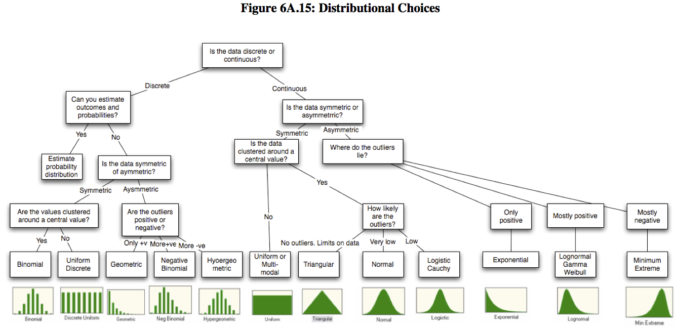
Aswath Damodaran. Probabilistic approaches: Scenario analysis, decision trees and simulations (PDF, the appendix is also available separately) and includes the following chart for choosing a distribution: