This is a failed attempt to simplify the process to generate multivariate Gaussian distribution by utilizing the copula function. However, it has the merit of figuring out what information a copula function failed to provide.
What is a copula function?
Copula is to describe the correlation of random variables. If we have a vector of RVs \((X_1, X_2, \cdots, X_d)\), each has a continuous CDF \(F_i(x)=\Pr[X_i\le x]\), then after integral transform on the RV vector, we have
\[(U_1, U_2, \cdots, U_d) = (F_1(X_1), F_2(X_2), \cdots, F_d(X_d))\]which is a vector over \([0,1]^d\) with each \(U_i\in[0,1]\). A copula \(C: [0,1]^d\mapsto [0,1]\) is the joint CDF:
\[\begin{align} C(\mathbf{u}) &= C(F_1(x_1), \cdots, F_d(x_d)) \\ &= C(u_1, u_2, \cdots, u_d) \\ &= \Pr[U_1\le u_1, U_2\le u_2, \cdots, U_d\le u_d] \end{align}\]Wikipedia mention that it has the properties:
- \(C(u_1, \cdots, u_{n-1}, 0, u_{n+1}, \cdots, u_d) = 0\), i.e., \(C(\mathbf{u})=0\) if any argument is 0
- \(C(1, \cdots, 1, u_n, 1, \cdots, 1) = u_n\), i.e., \(C(\mathbf{u})=u_n\) if all arguments are 1 except \(u_n\)
- \(C\) is non-decreasing, i.e.,
where \(B = \times_{i=1}^d [u_i,v_i]\) is any hyper-rectangle within \([0,1]^d\), \(\mathbf{z}\) of the summation goes over all corners of \(B\) (example of a corner: \((u_0, u_1, v_2, \cdots, u_{d-1}, v_d)\), i.e. each element of \(\mathbf{z}\) takes either the lower or upper bound in the dimension of the hyper-rectangle), and \(N(\mathbf{z})=\vert\{k: z_k=u_k\}\vert\) counts the number of element in vector \(\mathbf{z}\) that takes the lower bound in its dimension.
Use a bivariate as an example, \(C: [0,1]\times[0,1]\mapsto[0,1]\) and \(B=[0.5,0.6]\times[0.3,0.4]\), then
\[\int_B dC(\mathbf{u}) = (-1)^2 C(0.5, 0.3) + (-1)^1 C(0.5,0.4) + (-1)^1 C(0.6, 0.3) + (-1)^0 C(0.6, 0.4)\]After all, a copula function is just a probability distribution function. If we define the copula’s density
\[c = \frac{\partial^d C}{\partial F_1 \cdots \partial F_d}\]then the joint density function is related to the copula density by
\[f(\mathbf{x}) = c(F_1(x_1), \cdots, F_d(x_d)) \prod_{i=1}^d f_i(x_i)\]i.e., we can now calculate the joint density as if the RVs are independent of each other than multiply with the copula density.
Different kinds of copula functions
There are several kinds of copula functions, depends on how the \(C\) is based on. For example, a Gaussian copula has the form of
\[C_R^{\textrm{Gauss}}(\mathbf{u}) = \Phi_R(\Phi^{-1}(u_1),\cdots,\Phi^{-1}(u_d))\]which \(R\in[-1,1]^{d\times d}\) is the correlation matrix of the RVs, and \(\Phi^{-1}\) is the inverse CDF of standard normal distribution, and \(\Phi_R\) is the joint CDF of a multivariate normal distribution with mean vector of zero and covariance matrix \(R\), which therefore the copula’s density function is:
\[\begin{align} c_R^{\textrm{Gauss}}(\mathbf{u}) &= \frac{\partial^d C}{\partial\Phi_1\cdots\partial\Phi_d} \\ &= \frac{1}{\sqrt{\det R}}\exp\left( -\frac{1}{2} \begin{pmatrix} \Phi^{-1}(u_1) \\ \vdots \\ \Phi^{-1}(u_d) \end{pmatrix}^T (R^{-1}-I) \begin{pmatrix} \Phi^{-1}(u_1) \\ \vdots \\ \Phi^{-1}(u_d) \end{pmatrix} \right) \end{align}\]This compares to the general \(d\)-variate normal density function:
\[f(\mathbf{x}) = \left[ (2\pi)^{d/2} \prod_{i=1}^d \sqrt{\sigma_i\det R} \right]^{-1} \exp\left(-\frac12 \mathbf{z}^T R^{-1} \mathbf{z} \right)\]In other words, a Gaussian copula is a multivariate standard normal distribution function with correlation matrix \(R\), which each margin \(u_k\) has the probability integral transform \(\Phi^{-1}(u_k)\) applied.
Note that a Gaussian copula does not limit to multivariate Gaussian random variables \(\mathbf{X}\), as long as we can find the corresponding distribution \(\mathbf{u}\) (e.g. all are continuous) and the correlation \(R\) is well-defined.
Another copula function is the Achimedean copula, which is in the form of
\[C(\mathbf{u};\theta) = \psi^{[-1]}(\sum_{i=1}^d\psi(u_i;\theta);\theta)\]where \(\theta\in\Theta\) is a parameter, \(\psi:[0,1]\times\Theta\mapsto[0,\infty)\) is a continuous strictly decreasing convex function, known as the generator function, with \(\psi(1;\theta)=0\), and \(\psi^{[-1]}\) is its pseudo-inverse which \(\psi^{[-1]}(t;\theta) = \psi^{-1}(t;\theta)\) for \(0\le t\le \psi(0;\theta)\) and \(\psi^{[-1]}(t;\theta) = 0\) otherwise.
Expectation for copula models and Monte Carlo integration
Assume we have a function \(g: \mathbb{R}^d\mapsto\mathbb{R}\) and we are interested in \(E[g(\mathbf{X})]\) for some random vector \(\mathbf{X} = (X_1,\cdots,X_d)\). If the CDF of this random vector is \(H\), then
\[\begin{align} E[g(\mathbf{X})] &= \int_{\mathbb{R}^d} g(\mathbf{X}) dH(\mathbf{X}) \\ &= \int_{[0,1]^d} g(F_1^{-1}(u_1),\cdots,F_d^{-1}(u_d)) dC(\mathbf{u}) \\ &= \int_{[0,1]^d} g(F_1^{-1}(u_1),\cdots,F_d^{-1}(u_d)) c(\mathbf{u})du_1\cdots du_d \end{align}\]which the second equality arises if we have a copula model
\[H(x_1,\cdots,x_d)=C(F_1(x_1),\cdots,F_d(x_d))\]and the third equality arises if the copula \(C(\mathbf{u})\) is continuous and has a density function \(c(\mathbf{u})\). Substitute back \(u_i = F_i(x_i)\), and assuming the density \(f_i()\) is known, we have
\[E[g(\mathbf{X})] = \int_{\mathbb{R}^d} g(x_1,\cdots,x_d) c(F_1(x_1),\cdots,F_d(x_d))f_1(x_1)\cdots f_d(x_d)dx_1\cdots dx_d\]Which we can find the expectation using Monte Carlo algorithm:
- Draw \(n\) samples \(\mathbf{u}^{(k)}\) from copula function \(C(\mathbf{u})\)
- Produce samples \(\mathbf{X}^{(k)} = (X_1^{(k)},\cdots,X_d^{(k)}) = (F_1^{-1}(u_1^{(k)}),\cdots,F_d^{-1}(u_d^{(k)})) \sim H(\mathbf{x})\) from each \(\mathbf{u}^{(k)}\)
- Evaluate \(E[g(\mathbf{X})] = \frac{1}{n}\sum_{k} g(\mathbf{X}^{(k)})\)
Conversely, if we collected \(n\) samples of \(\mathbf{X}\), \((X_1^{(k)},X_2^{(k)},\dots,X_d^{(k)})\), the corresponding copula observations are \((F_1(X_1^{(k)}),F_2(X_2^{(k)}),\dots,F_d(X_d^{(k)}))\). We can approximate \(F_i(x)\) by empirical distribution \(F'_i(x) = \frac{1}{n}\sum_{k=1}^n 1_{X_i^{(k)} \le x}\) and corresponding empirical copula is therefore
\[C'(u_1,\cdots,c_d) = \frac{1}{n}\sum_{k=1}^n 1_{F'_1(X_1^{(k)})\le u_1, \cdots, F'_d(X_d^{(k)})\le u_d}\]Generating random vectors from a Gaussian copula
If we have a Gaussian copula \(C_R(\mathbf{u})\), we can generate random vectors from it using the following procedure:
- Perform Cholesky decomposition of the correlation matrix \(R=AA^T\) where \(A\) is the lower triangular matrix
- Generate a \(d\)-dimensional iid standard normal vector \(\mathbf{z}\)
- Multivariate normal random vector to generate is then \(\mathbf{x} = A\mathbf{z}\), with the corresponding copula vector \(\mathbf{u} = (\Phi(x_1), \cdots, \Phi(x_d))\)
This is exactly the same procedure to generate multivariate Gaussian random variables from the covariance matrix \(\Sigma\), only this time we use correlation matrix \(R\) instead. That makes sense because \(\Sigma\) and \(R\) are related:
\[R = (diag(\Sigma))^{-1/2} \Sigma (diag(\Sigma))^{-1/2}\]that is, diagonal of \(R\) is always 1 and off-diagonal terms are \(\frac{E[(X_i-\mu_i)(X_j-\mu_j]}{\sigma(X_i)\sigma(X_j)}=\frac{\sigma_{ij}}{\sigma_i\sigma_j}\)
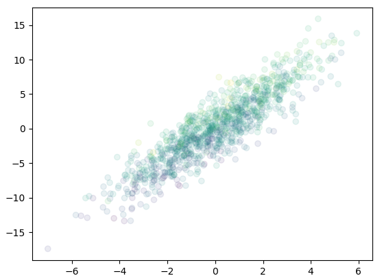
Up to here, we can see that the copula lost the information of mean and variance of individual components \(X_i\) of \(\mathbf{X}\), as it focus only on their correlation. The random vector generated from the copula is not the same as the original distribution, but scaled and shifted. This can be seen from the following plot:
# 3D gaussian random variable, generate from covariance matrix
from mpl_toolkits.mplot3d import Axes3D
import matplotlib.pyplot as plt
import numpy as np

Sigma = np.array([[4, 9, 3], [9, 25, 12], [3, 12, 25]])
S = np.linalg.cholesky(Sigma) # lower triangular part, i.e. S * S' == Sigma
iidnorm = np.random.randn(3,1000)
mvnorm = np.matmul(S, iidnorm)

fig = plt.figure()
ax = fig.add_subplot(111)
ax.scatter(mvnorm[0], mvnorm[1], c=mvnorm[2], alpha=0.1)
plt.show()
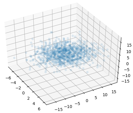
or equiv 3D scatter plot:
fig = plt.figure()
ax = fig.add_subplot(111, projection='3d')
ax.scatter(mvnorm[0], mvnorm[1], mvnorm[2], alpha=0.1)
plt.show()
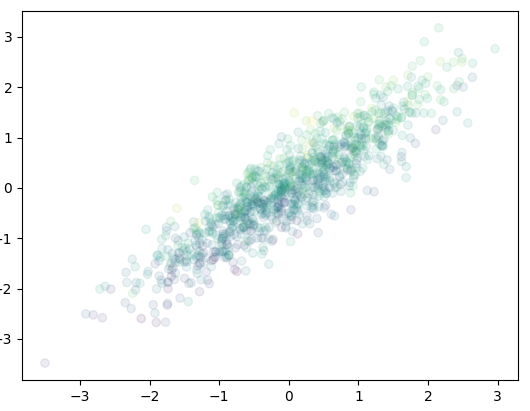
and the following is the same plot using Gaussian copula function (i.e. using the correlation matrix):
# From Sigma, generate the correlation matrix R
# Convert the covariance matrix into correlation matrix
SD = np.mat(np.sqrt(np.diag(Sigma))) # sqrt of diag vector, i.e. std dev
R = np.array(Sigma/np.multiply(D, D.T))
A = np.linalg.cholesky(R)
mvnorm = np.matmul(A, iidnorm)

fig = plt.figure()
ax = fig.add_subplot(111)
ax.scatter(mvnorm[0], mvnorm[1], c=mvnorm[2], alpha=0.1)
plt.show()
and the 3D version:
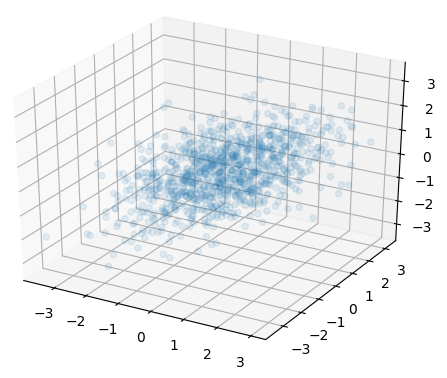
So we see, using the correlation matrix to generate the random vectors is like transforming the version of using covariance matrix to standard normal, as we lost the information of relative scale of variance in each dimension. Because of this, we do not make it any easier to generate multivariate random variables using copula function.
References
- https://ieeexplore.ieee.org/document/4419639 (DOI 10.1109/WSC.2007.4419639)
- http://www-1.ms.ut.ee/tartu07/presentations/zezula.pdf