Recently I encountered a problem of mixed integer programming with linear constraints but non-linear convex objective function. There do not seem to have any nice solver package available in Python. Even if I tried to look for anything with a C/C++ API, there are not many open source solutions, AFAIK. Therefore my second attempt is to solve the problem heuristically. It turns out the problem structure may allow a simple hill climbing (i.e., greedy search algorithm). However, while the objective function is convex, I cannot prove the solution domain is contiguous in all cases, hence I cannot guarantee there will not be any local minima. So play safe and use simulated annealing can be a good move.
Simulated annealing is a metaheuristic algorithm which means it depends on a handful of other parameters to work. But a simple skeleton algorithm is as follows:
def simulated_annealing(s0, k_max):
    s = s0
    for k in range(k_max):
        T = temperature(k/k_max)
        s_new = neighbour(s)
        if P(E(s), E(s_new), T) >= random.random():
            s = s_new
    return s
It starts searching with an initial solution s0 at temperature k_max, and
depends on an annealing schedule temperature(r). It keeps looking for a
randomly chosen neighbour(s) and accept such neighbour by a probability
function P(), which in turn depends on the energy level E() of solutions.
The acceptance probability function (e.g., in Metropolis-Hastings algorithm) is
exponential \(P(e, e', T) = \exp(-\frac{e'-e}{T})\) for \(e,e'\) to be the
energy level of s and its neighbour respectively. The function P() may
raise above 1 if the neighbour of s has lower energy (i.e. better) and in
such case the neighbour is accepted deterministically.
Variations of algorithm
Because simulated annealing is a metaheuristic algorithm, there are many variations available. A paper, Adaptive simulated annealing (ASA): Lessons learned, gave a very concise summary.
The original simulated annealing is modeled after Boltzmann equation. Thus named as Boltzmann Annealing (BA). It has a solution modelled as a \(d\)-vector \(x=(x^1, \cdots, x^d)\) with the annealing schedule \(T(k)=T_0/\log k\) for \(k\) denote the step count. It search a solution space by the probability density
\[g_T(\Delta x) = (2\pi T)^{-d/2}\exp\left(-\frac{\Delta x^2}{2T}\right)\]where \(\Delta x = x_{k+1} - x_k\) which usually \(x_k\) is the current solution and \(x_{k+1}\) is the neighbour. This is modelling the class of physical systems that called the Gaussian-Markovian systems. And the acceptance probability function is
\[h_T(\Delta E) = \frac{1}{1+\exp(\Delta E/T)} \approx \exp(-\Delta E/T)\]where \(\Delta E = E_{k+1}-E_k\) and this is also the form of probability function mentioned above. The Boltzmann Annealing is characterized by the annealing schedule \(T(k)\). It is proved that with such schedule, any point in the solution space can be sampled infinitely often in annealing time, i.e., \(\lim_{k\to\infty}\sum_k g_k = \infty\), or the sampling is ergodic.
If we switch to use the exponential schedule
\[T(k) = cT(k-1) = T_0 e^{(c-1)k}\]this will make the annealing faster but violates the assumption of ergodic sampling in BA. But people find this useful and named this as simulated quenching. Such schedule is also called the exponential cooling scheme (ECS).
Another variation is to use the Cauchy distribution for solution probability density:
\[g_T(\Delta x) = \frac{T}{(\Delta x^2 + T^2)^{(d+1)/2}}\]which has a fatter tail than the Gaussian distribution as in BA. Therefore, it is easier to get around the local minima while searching for the global minima. However, such density allows statistically same ergodicity as BA if the annealing schedule is \(T(k) = T_0/k\)., due to
\[\lim_{k\to\infty}\sum_k g_k = \frac{T_0}{\Delta x^{d+1}}\sum_k\frac{1}{k} = \infty\]Therefore, it is faster while similarly effective. This one is called fast annealing (FA).
Adaptive Simulated Annealing (ASA) is a further extension that allows each component \(x^i\) of the solution vector \(x\) to take a different domain, with different density function, and undergo a different annealing schedule. This expands the number of parameters to the algorithm to many folds.
Constrained optimization
The literature of simulated annealing usually do not explicitly concern about constrained optimization. One way to apply SA to constrained optimization is to implement the logic in the neighbour function so that each neighbour used is always within constrain. Another way is to implement the constrain in the objective function as penalties, e.g.
\[E^{\ast}(x) = E(x) + \frac{1}{T}\sum_i w_i c_i(x)\]for each \(c_i(x)\) the magnitude of violation in constrain \(i\) and \(w_i\) the corresponding weight in penalty. This approach may not be a good one especially if the valid solutions are sparse.
Parameter estimation
SA algorithm is mostly controlled by the temperate and its annealing schedule.
The well-received believe is that the initial temperature should be set to such a level that there is at least 80% probability to accept an increase in the objective function. And during the last 40% of annealing time, the algorithm should search in proximity of the optimal solution. One way to find the initial temperature \(T_0\) is to estimate (or observe) the average objective increase \(\Delta E^+\) and then set \(T_0 = -\frac{\Delta E^+}{\log p_0}\) for the initial probability of acceptance (e.g., \(p_0 = 0.8\)).
The annealing schedule can also be fine-tuned such that there can be more than one neighbour searched in every temperature step \(k\). Indeed, for a fixed temperature, the search and transition between neighbours forms a Markov Chain. We can designate a maximum length \(L_k\) for a Markov Chain at step \(k\) such that we either check a total of \(L_k\) solutions or accepted \(N_{min} \le L_k\) solutions, then the temperate should be decreased for one step.
Sudoku
I found a Python package simanneal for simulated annealing. SA algorithm is simple enough that we can code our own, this package may not be an absolute necessary. However, it is simple enough to use. Let’s start with the code:
#!/usr/bin/env python

import copy
import random
from simanneal import Annealer

# from https://neos-guide.org/content/sudoku
_ = 0
PROBLEM = [
    1, _, _,  _, _, 6,  3, _, 8,
    _, _, 2,  3, _, _,  _, 9, _,
    _, _, _,  _, _, _,  7, 1, 6,

    7, _, 8,  9, 4, _,  _, _, 2,
    _, _, 4,  _, _, _,  9, _, _,
    9, _, _,  _, 2, 5,  1, _, 4,

    6, 2, 9,  _, _, _,  _, _, _,
    _, 4, _,  _, _, 7,  6, _, _,
    5, _, 7,  6, _, _,  _, _, 3,
]

def print_sudoku(state):
    border = "------+------+------"
    rows = [state[i:i+9] for i in range(0,81,9)]
    for i,row in enumerate(rows):
        if i % 3 == 0:
            print(border)
        three = [row[i:i+3] for i in range(0,9,3)]
        print(" |".join(
            " ".join(str(x or "_") for x in one)
            for one in three
        ))
    print(border)

def init_solution_row(problem):
    """Generate a random solution from a Sudoku problem
    """
    solution = []
    for i in range(0, 81, 9):
        row = problem[i:i+9]
        permu = [n for n in range(1,10) if n not in row]
        random.shuffle(permu)
        solution.extend([n or permu.pop() for n in row])
    return solution

def coord(row, col):
    return row*9 + col

class Sudoku_Row(Annealer):
    def __init__(self, problem):
        self.problem = problem
        state = init_solution_row(problem)
        super().__init__(state)
    def move(self):
        """randomly swap two cells in a random row"""
        row = random.randrange(9)
        coords = range(9*row, 9*(row+1))
        n1, n2 = random.sample([n for n in coords if self.problem[n] == 0], 2)
        self.state[n1], self.state[n2] = self.state[n2], self.state[n1]
    def energy(self):
        """calculate the number of violations: assume all rows are OK"""
        column_score = lambda n: -len(set(self.state[coord(i, n)] for i in range(9)))
        square_score = lambda n, m: -len(set(self.state[coord(3*n+i, 3*m+j)] for i in range(3) for j in range(3)))
        return sum(column_score(n) for n in range(9)) + sum(square_score(n,m) for n in range(3) for m in range(3))

def coord(row, col):
    return row*9+col

def main():
    sudoku = Sudoku_Row(PROBLEM)
    sudoku.copy_strategy = "slice"
    sudoku.steps = 1000000
    print_sudoku(sudoku.state)
    state, e = sudoku.anneal()
    print("\n")
    print_sudoku(state)
    print(e)

if __name__ == "__main__":
    main()
Instead of try with the traditional unconstrained continuous minimization
problem, we go with an unnatural choice of a constrained combinatorial problem.
We pick the sudoku problem from https://neos-guide.org/content/sudoku, and
use the simanneal module. The implementation is easy: Just derive a class
from Annealer and define two member functions move() and energy(), for
neighbour search and objective function to minimize respectively. The SA
algorithm should start with initializing the Annealer with an initial
solution and call anneal() to get the optimal state variable and its
corresponding energy level.
The above program try to find a permutation of 1 to 9 in each row and check if it comes up with a solution to the sudoku problem. Every step is to pick a row in the original state and swap two positions. The energy function is to count the number of distinct elements in each row and square block and take the negation of the sum. A perfect solution will be \(-9\times 9\times 2 = -162\). This program does not work well. It does not come up with a correct solution. So my second attempt is not to shuffle by row but by square blocks:
import copy
import random
import numpy as np
from simanneal import Annealer

# from https://neos-guide.org/content/sudoku
_ = 0
PROBLEM = np.array([
    1, _, _,  _, _, 6,  3, _, 8,
    _, _, 2,  3, _, _,  _, 9, _,
    _, _, _,  _, _, _,  7, 1, 6,

    7, _, 8,  9, 4, _,  _, _, 2,
    _, _, 4,  _, _, _,  9, _, _,
    9, _, _,  _, 2, 5,  1, _, 4,

    6, 2, 9,  _, _, _,  _, _, _,
    _, 4, _,  _, _, 7,  6, _, _,
    5, _, 7,  6, _, _,  _, _, 3,
])

def print_sudoku(state):
    border = "------+-------+------"
    rows = [state[i:i+9] for i in range(0,81,9)]
    for i,row in enumerate(rows):
        if i % 3 == 0:
            print(border)
        three = [row[i:i+3] for i in range(0,9,3)]
        print(" | ".join(
            " ".join(str(x or "_") for x in one)
            for one in three
        ))
    print(border)

def coord(row, col):
    return row*9+col

def block_indices(block_num):
    """return linear array indices corresp to the sq block, row major, 0-indexed.
    block:
       0 1 2     (0,0) (0,3) (0,6)
       3 4 5 --> (3,0) (3,3) (3,6)
       6 7 8     (6,0) (6,3) (6,6)
    """
    firstrow = (block_num // 3) * 3
    firstcol = (block_num % 3) * 3
    indices = [coord(firstrow+i, firstcol+j) for i in range(3) for j in range(3)]
    return indices

def initial_solution(problem):
    """provide sudoku problem, generate an init solution by randomly filling
    each sq block without considering row/col consistency"""
    solution = problem.copy()
    for block in range(9):
        indices = block_indices(block)
        block = problem[indices]
        zeros = [i for i in indices if problem[i] == 0]
        to_fill = [i for i in range(1, 10) if i not in block]
        random.shuffle(to_fill)
        for index, value in zip(zeros, to_fill):
            solution[index] = value
    return solution

class Sudoku_Sq(Annealer):
    def __init__(self, problem):
        self.problem = problem
        state = initial_solution(problem)
        super().__init__(state)
    def move(self):
        """randomly swap two cells in a random square"""
        block = random.randrange(9)
        indices = [i for i in block_indices(block) if self.problem[i] == 0]
        m, n = random.sample(indices, 2)
        self.state[m], self.state[n] = self.state[n], self.state[m]
    def energy(self):
        """calculate the number of violations: assume all rows are OK"""
        column_score = lambda n: -len(set(self.state[coord(i, n)] for i in range(9)))
        row_score = lambda n: -len(set(self.state[coord(n, i)] for i in range(9)))
        score = sum(column_score(n)+row_score(n) for n in range(9))
        if score == -162:
            self.user_exit = True # early quit, we found a solution
        return score

def main():
    sudoku = Sudoku_Sq(PROBLEM)
    sudoku.copy_strategy = "method"
    print_sudoku(sudoku.state)
    #sudoku.steps = 1000000
    #auto_schedule = sudoku.auto(minutes=1)
    #print(auto_schedule)
    #sudoku.set_schedule(auto_schedule)
    sudoku.Tmax = 0.5
    sudoku.Tmin = 0.05
    sudoku.steps = 100000
    sudoku.updates = 100
    state, e = sudoku.anneal()
    print("\n")
    print_sudoku(state)
    print("E=%f (expect -162)" % e)

if __name__ == "__main__":
    main()
This version is to find a neighbour by picking a square
block randomly and swap two positions in it. Therefore each block is guaranteed
to have 1 to 9 but we have to check each row and column for consistency. We
also add assert self.user_exit when a solution is found so we can have a
early termination. The performance is only slightly better (or may be not, I
didn’t collect enough statistics to claim this). And neither program ever find
a solution.
However, if we try to use the auto() function to find the schedule (the
commented lines in main() above), the program start to find a solution,
albeit not always. A few other modification increased the chance of reaching a
solution:
Firstly, in simanneal module, the temperature update is based on this formula:
T = self.Tmax * math.exp(Tfactor * step / self.steps)
where Tfactor is a constant derived from Tmax and Tmin so that it
guarantees the temperate T goes from Tmax to Tmin over the annealing
schedule. It turns out the normal setting is having the temperature dropping
too fast. This is an adverse effect to the search that trap us in a sub-optimal
solution. If we change this to T = 0.99999 * T, it will be easier to reach a
solution. But we can achieve the same by gauging Tmax and Tmin to closer to
each other, so we have the second modification:
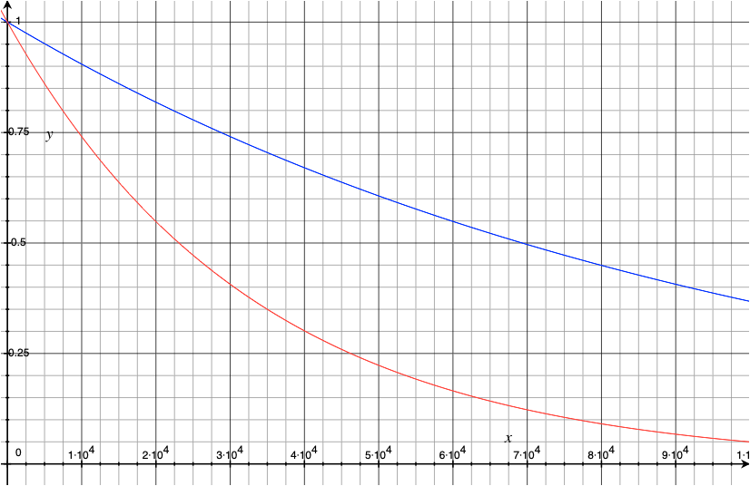
Secondly, we set some particular number for Tmax and Tmin (also steps).
They are found empirically such that a solution can be reached in a few seconds
instead of minutes. It turns out a low Tmax and comparable Tmin can
maintain a good effectiveness by keeping the temperature decrease steady. The
following chart shows the annealing schedule according to the exponential decay
formula in simanneal above, scaled to match the starting point at step 0. The
blue curve is using the value 0.5 and 0.05 respectively, as in the code above.
The red curve is the default value of 2500 and 2.5 respectively. The absolute
value of T does not matter in this chart but the ratio of Tmax and Tmin
do. The value of T, however, plays a role in the probability function of
acceptance and thus it set as such.
How about SA with constant temperature? Make Tmin and Tmax equal. How
about simple hill-climbing instead of SA? Set Tmax to as close to zero as
possible so the acceptance probability function is virtually 0. But a problem
of combinatorial nature should not be suitable for hill-climbing search.
Reference
Lester Ingber, Adaptive simulated annealing (ASA): Lessons learned. Control and Cybernetics, 1995. arXiv:cs/0001018
Franco Busetti, Simulated annealing overview