I was introduced to the concept of self-similarity and long-range dependency of a time series from the seminal paper On the Self-Similar Nature of Ethernet Traffic by Leland et al (1995). The Hurst parameter or the Hurst exponent is the key behind all these.
If we consider a Brownian motion, regardless of scale, we always have the property that the standard deviation of the process is proportional to the square root of time, namely, \(B_t - B_s \sim N(0, t-s)\) in distribution. The Brownian motion is memoryless, hence no long-range dependency. When we generalize the Brownian motion, we can consider a zero-mean process \(B_H(t)\) with the property
\[\langle\vert B_H(t+\tau) - B_H(t)\vert^2\rangle \sim \tau^{2H}\]namely, the mean of the square difference is proportional to the time window to the power of \(2H\). The range of \(H\) is from 0 to 1 and Brownian motion has \(H=0.5\). The parameter \(H\) is the Hurst exponent. Fractal dimension is defined in terms of Hurst exponent as \(D=2-H\).
In J. Feder’s book Fractals (1998), it accounts for how Hurst calculate the Hurst exponential for the water level in Lake Albert. Hurst denotes the influx of year \(t\) as \(\xi(t)\) and the discharge as \(\langle\xi\rangle_\tau\), which
\[\langle\xi\rangle_\tau = \frac{1}{\tau}\sum_{t=1}^\tau \xi(t)\]The accumulation is therefore the running sum
\[X(t)=\sum_{u=1}^t\left(\xi(u)-\langle\xi\rangle_\tau\right)\]The range is defined as
\[R(\tau) = \max_{t: t=1,\cdots,\tau} X(t) - \min_{t: t=1,\cdots,\tau} X(t)\]and the standard deviation is defined as
\[S=\sqrt{\frac{1}{\tau}\sum_{t=1}^\tau\left(\xi(t)-\langle\xi\rangle_\tau\right)^2}\]Hurst found that, \(R/S=(\tau/2)^H\), which the LHS is called the rescaled range and it is proportional to \(\tau^H\). This can be understood intuitively if we consider the range is roughly a measure to the standard deviation, which its square is the variance and is proportional to \(\tau^{2H}\).
Determining Hurst exponent
If we are given a time series \(X(t)\), how could we find its Hurst exponent (and hence tell if it is Brownian)?
The intuitive way is using Hurst’s empirical method: With different time ranges \(\tau\), find the rescaled range \(R/S\) and then fit for the parameter \(H\) using \(R/S = C\tau^H\) for some constant \(C\). But as the time ranges \(\tau\) varies, we may be able to fit multiple windows in the input time series. Hence multiple rescaled range can be computed, and we can take the average for the particular \(\tau\).
Here is the code:
def hurst_rs(ts, min_win=5, max_win=None):
    """Find Husrt exponent using rescaled range method

    Args:
        ts: The time series, as 1D numpy array
        min_win: Minimum window to use
        max_win: Maximum window to use
    Return:
        Hurst exponent as a float
    """
    ts = np.array(ts)
    max_win = max_win or len(ts)
    win = np.unique(np.round(np.exp(np.linspace(np.log(min_win), np.log(max_win), 10))).astype(int))
    rs_w = []
    for tau in win:
        rs = []
        for start in np.arange(0, len(ts)+1, tau)[:-1]:
            pts = ts[start:start+tau] # partial time series
            r = np.max(pts) - np.min(pts) # range
            s = np.sqrt(np.mean(np.diff(pts)**2)) # RMS of increments as standard deviation
            rs.append(r/s)
        rs_w.append(np.mean(rs))
    p = np.polyfit(np.log(win), np.log(rs_w), deg=1)
    return p[0]
The function would not find the rescaled range for all time window \(\tau\)
because it is too slow for practical use. Instead, it evenly takes 10 points in
the log scale from the minimum to the maximum. For each \(\tau\), np.arange(0,
len(ts)+1, tau) generates starting points separated by one full window, hence
we partitioned the time series into non-overlapping sequences of length tau,
except the last one, which the input time series may run out, and hence
discarded. Then for each partiel time series, a range is found and the
root-mean-squared increment is considered as standard deviation (since we
assumed the increments are having zero mean). For each \(\tau\), the \(R/S\) is
taken as the mean of all rescaled ranges from different partial time series. Then we consider
and hence a linear regression (degree-1 polynomial) fitting \(\log(R/S)\) against \(\log(\tau)\) will produce the Hurst exponent as the order-1 coefficient.
Another method is to use the scaling properties of a fBm:
def hurst_sp(ts, max_lag=50):
    """Returns the Hurst Exponent of the time series using scaling properties"""
    lags = range(2, max_lag)
    ts = np.array(ts)
    stdev = [np.std(ts[tau:]-ts[:-tau]) for tau in lags]
    p = np.polyfit(np.log(lags), np.log(stdev), 1)
    return p[0]
This is a much shorter code but it considered \(B_H(t+\tau)-B_H(t)\), which its standard deviation is expected to be proportional to \(\tau^H\). The difference is computed directly across the entire time series and then the standard deviation is computed. Then, as before, we fit a linear equation between the time lag and the standard deviation of the difference, and the Hurst exponent is the order-1 coefficient.
It turns out, I found that the rescaled range method often overestimate the Hurst exponent and the scaling property method sometimes underestimates. As seen below:
N = 2500
sigma = 0.15
dt = 1/250.0
bm = np.cumsum(np.random.randn(N)) * sigma / (N*dt)
h1 = hurst_rs(bm)
h2 = hurst_sp(bm)
print(f"Hurst (RS):      {h1:.4f}")
print(f"Hurst (scaling): {h2:.4f}")
print(f"Hurst (average): {(h1+h2)/2:.4f}")
This gives
Hurst (RS):      0.5927
Hurst (scaling): 0.4783
Hurst (average): 0.5355
Generating fractional Brownian motion
What if we are given \(H\) and generate a time series? This is more difficult then it seems. The Hurst exponent is ranged from 0 to 1, with Brownian motion is \(H=0.5\). If \(H<0.5\), the time series is mean-reverting, and if \(H>0.5\), the time series is trending or with long-range dependency (LRD). The other way to understand this is that, if \(H>0.5\), the increments are positively correlated, while \(H<0.5\) then they are negatively correlated.
Wikipedia gives a few property of the fractional Brownian motion:
- self-similarity: \(B_H(at) \sim \vert a\vert^H B_H(t)\)
- stationary increment: \(B_H(t)-B_H(s) = B_H(t-s)\)
- long range dependency: if \(H>0.5\), we have \(\sum_{k=1}^\infty \mathbb{E}[B_H(1)(B_H(k+1)-B_H(k))] = \infty\)
- regularity: for any \(\epsilon>0\), there exists constant \(c\) such that \(\vert B_H(t) - B_H(s)\vert \le c\vert t-s\vert^{H-\epsilon}\)
- covariance of increment of \(B_H(s)\) and \(B_H(t)\) is \(R(s,t) = \frac12(s^{2H}+t^{2H}-\vert t-s\vert^{2H})\)
We can based on the covariance of increment to create a huge covariance matrix (each row and column corresponds to one time sample) and use the Cholesky decomposition method to generate correlated Gaussian samples. The fBm is the running sum of these samples.
Another way to generate this is as follows, adopted from a MATLAB code:
def fbm1d(H=0.7, n=4096, T=10):
    """fast one dimensional fractional Brownian motion (FBM) generator
    output is 'W_t' with t in [0,T] using 'n' equally spaced grid points;
    code uses Fast Fourier Transform (FFT) for speed.
    Adapted from http://www.mathworks.com.au/matlabcentral/fileexchange/38935-fractional-brownian-motion-generator

    Args:
        H: Hurst parameter, in [0,1]
        n: number of grid points, will be adjusted to a power of 2 by n:=2**ceil(log2(n))
        T: final time
    Returns:
        W_t and t for the fBm and the time
    Example:
        W, t = fbm1d(H, n, T)
        plt.plot(t, W)
    Reference:
        Kroese, D. P., & Botev, Z. I. (2015). Spatial Process Simulation.
        In Stochastic Geometry, Spatial Statistics and Random Fields(pp. 369-404)
        Springer International Publishing, DOI: 10.1007/978-3-319-10064-7_12
    """
    # sanitation
    assert 0<H<1, "Hust parameter must be between 0 and 1"
    n = int(np.exp2(np.ceil(np.log2(n))))
    r = np.zeros(n+1)
    r[0] = 1
    idx = np.arange(1,n+1)
    r[1:] = 0.5 * ((idx+1)**(2*H) - 2*idx**(2*H) + (idx-1)**(2*H))
    r = np.concatenate([r, r[-2:0:-1]]) # First row of circulant matrix
    lamb = np.fft.fft(r).real/(2*n) # Eigenvalues
    z = np.random.randn(2*n) + np.random.randn(2*n)*1j
    W = np.fft.fft(np.sqrt(lamb) * z)
    W = n**(-H) * np.cumsum(W[:n].real) # rescale
    W = T**H * W
    t = np.arange(n)/n * T # Scale for final time T
    return W, t
The explanation of why this works is in the article referenced above. But we can see the plot as follows:
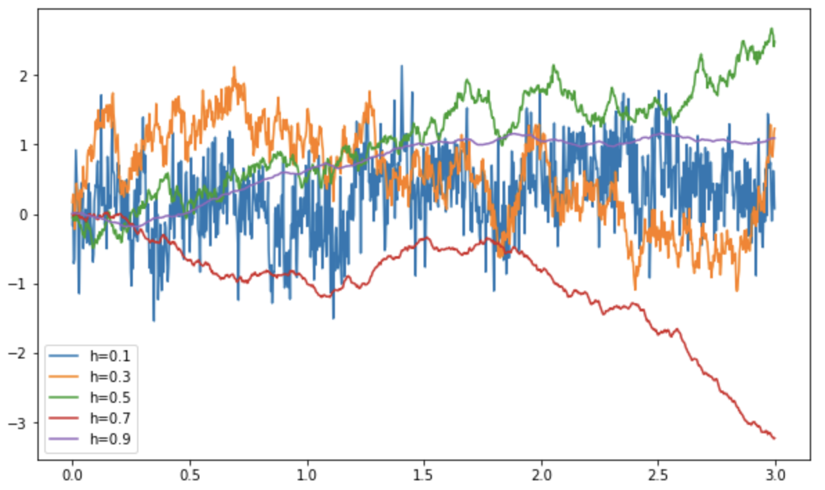
which we can see that the lower the Hurst exponent, the more fluctuating the random walk, and the higher the Hurst exponent, the smoother.