Gaussian Process Regression

Gaussian process regression is an interesting method of function regression. It is non-parametric, meaning not to assume anything (linear, polynomial, etc.) about the objective function. Let’s consider a function of \(\mathbb{R}\mapsto\mathbb{R}\). Without knowing anything or assuming anything, the fuction \(f(x)\) can take, and maps to, any value in \(\mathbb{R}\). We can simply model \(f(x)\sim N(0,1)\) for all \(x\) and consider what the Gaussian probability means later.

If \(f(x)\sim N(0,1)\) i.i.d. for any \(x\), this function is the Gaussian noise. Gaussian process assumes \(f(x)\) is not independent for different \(x\). If we consider only sample locations \((x_1, \cdots, x_d)\) and assume \(f(x_i)\) and \(f(x_j)\) are correlated with Pearson coefficient \(R_{ij}\), we can assume the correlation matrix to be \(\mathbf{K}\) (i.e., \(K_{ii}=1\) and \(K_{ij}=R_{ij}\)). Then

i.e., we modeled \(f(x)\) as zero-centered multivariate Gaussian with covariance matrix \(\mathbf{K}\).

In Gaussian process regression, we would assume some kernel function \(k(x_i, x_j) = R_{ij}\). A usual choice is the squared exponential,

which \(k(x_i, x_j)\) will run from 1 to 0 as \(x_i\) and \(x_j\) are further apart.

With such kernel function, we can generate multiple functions samples:

import numpy as np
import scipy.linalg
import scipy.stats
import scipy as sp
import matplotlib.pyplot as plt

def kernel(x1, x2, lam=1):
    """GP squared exponential kernel"""
    x1 = np.asarray(x1).reshape(-1,1)
    x2 = np.asarray(x2).reshape(1,-1)
    sqdist = (x1 - x2)**2
    return np.exp(-(0.5/lam)*sqdist)

LBOUND=-5
UBOUND=5
N_POINTS=50
M = 10

# Generate M random functions
x = np.linspace(LBOUND, UBOUND, N_POINTS)
K = kernel(x,x)
if "use scipy":
    y = sp.stats.multivariate_normal.rvs(np.zeros_like(x), K, size=M).T
else:
    # Will run into issue of K not positive definite due to numerical rounding
    # better to fix it by rounding small negative eigenvalues to zero
    # see https://www.r-bloggers.com/2012/10/fixing-non-positive-definite-correlation-matrices-using-r-2/
    L = sp.linalg.cholesky(K, lower=True, check_finite=False)
    z = np.random.randn(N_POINTS, M)
    y = (L @ z).T
plt.figure(figsize=(8,6))
plt.plot(x, y)
plt.show()

Using the multivariate normal random number generator from scipy should be preferred over the use of Cholesky decomposition due to the floating point rounding error. The script above does not specify the objective function. It will just give you a bunch of random curves:

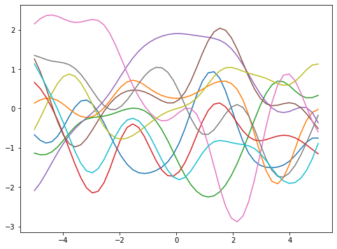
These are what we called the prior. These are what we can have before having any data. The hyperparameter \(\lambda\) in the kernel function controls how smooth the curves would be. The larger the \(\lambda\), the larger the correlation, hence the smoother the function.

Now if have data \((x_i, f(x_i))\) for \(i=1,\cdots,n\), and we are interested in the positions \(x^\ast_i\) for \(i=1,\cdots,m\), this model tells us that

where \(\mathbf{K}_\ast\) is the matrix of correlations computed using the kernel function from elements of \(\mathbf{x}\) and \(\mathbf{x}^\ast\), and \(\mathbf{K}_{\ast\ast}\) is the matrix of correlations computed using the kernel function amongst elements of \(\mathbf{x}^\ast\).

Since this is a multivariate Gaussian distribution, we can borrow some techniques. One particular technique is the posterior conditional. It says if we have

(which every element is a submatrix), then the conditional distribution is:

Since we have \(f(x_i)\) known and \(f(x_i^\ast)\) unknown, we can find the conditional distribution

for

Which in our model, \(\mu_\mathbf{x}=\mathbf{0}\) and \(\mu_{\mathbf{x}^\ast}=\mathbf{0}\).

The vector \(\mu\) is what we expect the \(f(x_i^\ast)\) to be (the mean over the function space) and the diagonal of \(\Sigma\) are the variances of \(f(x_i^\ast)\). The below is how we can chart the objective function as a family of functions.

# This is the true unknown function we are trying to approximate
f = lambda x: np.sin(0.9*x).flatten()

N_SAMPLE = 5

# Sample some input points
x_sample = np.random.uniform(LBOUND, UBOUND, size=(N_SAMPLE,))
y_sample = f(x_sample)

# Compute the kernel matrix
K = kernel(x_sample, x_sample)
Kss = kernel(x,x)
Ks = kernel(x_sample, x)
Kinv = np.linalg.inv(K)
Sigma = Kss - Ks.T @ Kinv @ Ks

# Compute location matrix
mu = Ks.T @ Kinv @ y_sample

# Compute standard deviations
sd = np.sqrt(np.diag(Sigma))

# Generate sample functions
y = sp.stats.multivariate_normal.rvs(mu, Sigma, size=M).T

# Plot
x_plot = np.append(x_sample, x)
y_plot = np.append(np.repeat(y_sample.reshape(-1,1), 10, axis=1), y, axis=0)
arg = np.argsort(x_plot)
plt.figure(figsize=(8,6))
plt.gca().fill_between(x, mu-2*sd, mu+2*sd, color="#dddddd", alpha=0.5)
plt.plot(x, mu, c="r")
plt.plot(x_plot[arg], y_plot[arg], alpha=0.5)
plt.scatter(x_sample, y_sample, c="r", alpha=0.5)
plt.show()

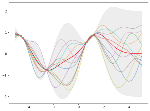
In this plot, we see that the nodes are at \(x_i\) as the value of \(f(x_i)\) are known and there are zero variances. The further aways from any \(x_i\), the larger the variance.

It is easy to extend this model to the case that the exact value of \(f(x_i)\) are unknown but we have estimates. Here we introduce the variance of estimates \(\sigma_y^2\) (a constant) and assume we estimated \(y_i = f(x_i) + \epsilon\) with \(\epsilon\sim N(0,\sigma_y^2)\).

If \(f(\mathbf{x}) \sim N(\mu, \mathbf{K})\), then by additive property of variance we have \(\mathbf{y} \sim N(\mu, \mathbf{K}+\sigma_y^2 \mathbf{I})\). So we have

Note that \(\mathbf{K}_\ast\) and \(\mathbf{K}_{\ast\ast}\) are same as previous (Gaussian noise is independent and hence covariance of \(f(x_j)\) and \(f(x_i^\ast)\) is same as covariance of \(y_j\) and \(f(x_i^\ast)\)). But now we have

for

The code to plot in this case is as follows:

# Function with noise
sigma_y = 5e-2
f_noise = lambda x: f(x) + sigma_y*np.random.randn(*x.shape)
y_noise = f_noise(x_sample)

# Compute the kernel matrix
Ky = kernel(x_sample, x_sample) + (sigma_y**2)*np.eye(N_SAMPLE)
Kss = kernel(x,x)
Ks = kernel(x_sample, x)
Kinv = np.linalg.inv(Ky)
Sigma = Kss - Ks.T @ Kinv @ Ks

# Compute location matrix
mu = Ks.T @ Kinv @ y_noise

# Compute standard deviations
sd = np.sqrt(np.diag(Sigma))

# Generate sample functions
y = sp.stats.multivariate_normal.rvs(mu, Sigma, size=M).T

# Plot
plt.figure(figsize=(8,6))
plt.gca().fill_between(x, mu-2*sd, mu+2*sd, color="#dddddd", alpha=0.5)
plt.plot(x, y, alpha=0.5)
plt.plot(x, mu, c="r")
plt.scatter(x_sample, y_sample, c="r", alpha=0.5)
plt.show()

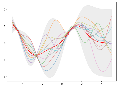
Which the above plot has non-zero (\(\sigma_y^2>0\)) variance at the nodes of \(x_i\). Moreover, the estimates \(y_i\) (red dots) are not always on the expectation \(\mu\) (red line). In fact, they are related as

Since \(\mathbf{K}\) and \(\mathbf{K}_\ast\) above are depending on the kernel function, in which a hyperparameter \(\lambda\) is involved in our squared exponential kernel. Varying \(\lambda\) will give us a different \(\mu\) (namely, the estimated function) as it controls how smooth the function would be.

If we consider only \(\mathbf{y} \sim N(\mu, \mathbf{K}+\sigma_y^2\mathbf{I}) = N(\mathbf{0}, \mathbf{K}+\sigma_y^2\mathbf{I})\), then

and if we consider the kernel parameter \(\lambda_{ij}\) is used on \(k(x_i,x_j)\) (which in the simplest case can be the same for all \(i,j\)), we can have the partial derivative

and we can apply gradient descent to find the optimial hyperparameter given the estimates \(\mathbf{y}\) at locations \(\mathbf{x}\).