Copula is a multivariate CDF defined over \(C: [0,1]^d \mapsto [0,1]\),
\[C(u_1,u_2,\cdots,u_d) = \Pr[U_1\le u_1, U_2\le u_2,\cdots,U_d\le u_d]\]for random vector \(\mathbf{U}=[U_1,U_2,\cdots,U_d]\).
Support on the unit hypersquare \([0,1]^d\) only. And a copula satisfies the properties:
\[\begin{aligned} C(1,1,\dots,1) &= 1 \\ C(\dots,u_i,0,u_{i+2},\dots) &= 0 \\ C(1,\dots,1,u,1,\dots,1) &= u \end{aligned}\]which the first two are intuitive from the definition of a multivariate CDF, and the last one gives the marginal distribution.
If \(C(u_1,u_2,\cdots,u_d)\) is a copula of dimension \(d\), then \(C(1,u_2,\cdots,u_d)\) is a copula of dimension \(d-1\).
If we have the function \(C\) well defined, the probability over the hyperrectangle \(B=[u_1,v_1]\times[u_2,v_2]\times\cdots\times[u_d,v_d]=\times_{i=1}^d[u_i,v_i]\) within \([0,1]^d\) is
\[\int_B dC(\mathbf{u})=\sum_{\mathbf{z}=\times_{i=1}^d\{u_i,v_i\}} (-1)^{N(\mathbf{z})}C(\mathbf{z})\]and \(N(\mathbf{z})\) is the count of the number of elements in \(\mathbf{z}\) that takes the lowerbound \(u_i\). For example, if \(d=2\), we have \(B=[u_1,v_1]\times[u_2,v_2]\) and
\[\int_B dC(\mathbf{u})=C(u_1,u_2)-C(u_1,v_2)-C(v_1,u_2)+C(v_1,v_2)\]Copula is a function to reveal correlation or dependency structure without providing the actual joint distribution. We can convert a copula and the marginal distributions of each component into a joint distribution using the Sklar’s theorem: For copula \(C(u,v)\) and marginal distributions \(u=F_X(x)\) and \(v=F_Y(y)\), the joint probability distribution is
\[F_{XY}(x,y) = C(F_X(x),F_Y(y))\]Copula, marginals, and distribution function
For a CDF \(F(x)\), the quantile function is the generalized inverse:
\[F^{\leftarrow}_X(u) := \inf\{x: F(x)\ge u\}\]and we have
\[\Pr[F^{\leftarrow}(u) \le x] = F_X(x)\]If \(F\) is continuous and monotonically increasing, the quantile function \(F^{\leftarrow} \equiv F^{-1}\) as the latter exists. In that case, \(F_X(x)\) is a random variable on Uniform(0,1).
For a random vector \(\mathbf{X}=(X_1,\cdots,X_d)\), which the marginals are \(F_{X_i}(x_i)\) and the joint distribution is \(F_{\mathbf{X}}(\mathbf{x})\), then we can transform \(\mathbf{X}\) into a vector of Uniform(0,1) random variables \(\mathbf{U}\), then find its copula using Sklar’s theorem:
\[\begin{aligned} & F_{\mathbf{X}}(x_1,\cdots,x_d) \\ =& F_{\mathbf{X}}(F^{\leftarrow}_{X_1}(u_1),\cdots,F^{\leftarrow}_{X_d}(u_d)) \\ =& \Pr[x_1\le F^{\leftarrow}_{X_1}(u_1), \cdots, x_d\le F^{\leftarrow}_{X_d}(u_d)] \\ =& \Pr[F_{X_1}(x_1)\le u_1, \cdots, F_{X_d}(x_d)\le u_d] \\ =& C_{\mathbf{X}}(u_1,\cdots,u_d) \end{aligned}\]Copula is invariant under monotonic transformation: For copula \(C_X(u_1,\dots,u_d)\) of \(X\), we have marginal distributions \(u_k = F_{X_k}(x_k)\). With \(y_k=T(x_k)\) for some monotonic function \(T(\cdot)\), there is a mapping of \(u_k=F_{Y_k}(y_k)=F_{Y_k}(T(x_k))\).
\[\begin{aligned} & C_{\mathbf{X}}(u_1,\cdots,u_d) \\ =& F_{\mathbf{X}}(F^{\leftarrow}_{X_1}(u_1),\cdots,F^{\leftarrow}_{X_d}(u_d)) \\ =& F_{\mathbf{X}}(T_1^{-1}(F^{\leftarrow}_{Y_1}(u_1)),\cdots,T_d^{-1}(F^{\leftarrow}_{Y_d}(u_d))) \\ =& F_{\mathbf{Y}}(F^{\leftarrow}_{Y_1}(u_1),\cdots,F^{\leftarrow}_{Y_d}(u_d)) \\ =& C_{\mathbf{Y}}(u_1,\cdots,u_d) \end{aligned}\]Now consider an example (Haugh, 2016), where \(Y,Z\sim F\) and \(X_1=\min(Y,Z)\), \(X_2=\max(Y,Z)\). The marginals are:
\[\begin{aligned} F_{X_1}(x) &= \Pr[X_1\le x] = \Pr[\min(Y,Z)\le x] \\ &= 2\int_{-\infty}^x dF(u)\int_u^\infty dF(v) \\ &= 2\int_{-\infty}^x dF(u)\Big(1-F(u)\Big) \\ &= 2\Big(F(x) - \int_{-\infty}^x F(u)dF(u)\Big) \\ &= 2\Big(F(x) - \frac12 F^2(x)\Big) \\ &= 2F(x) - F^2(x) \\ F_{X_2}(x) &= \Pr[X_2\le x] = \Pr[\max(Y,Z)\le x] \\ &= \Pr[Y\le x, Z\le x] \\ &= F^2(x) \end{aligned}\]and the joint distribution from copula:
\[C(u_1,u_2) = C(F_{X_1}(x_1),F_{X_2}(x_2)) = \Pr[X_1\le x_1, X_2\le x_2]\]if \(x_1\ge x_2\),
\[\begin{aligned} C(F_{X_1}(x_1),F_{X_2}(x_2)) &= \Pr[Y\le x_2, Z\le x_2] \\ &= F_{X_2}(x_2) \\ &= F^2(x_2) \end{aligned}\]if \(x_1\le x_2\),
\[\begin{aligned} C(F_{X_1}(x_1),F_{X_2}(x_2)) &= \Pr[Y\le x_1, x_1\le Z\le x_2] + \Pr[Z\le x_1, x_1\le Y\le x_2] \\ &= 2\int_{-\infty}^{x_1} dF(u) \int_u^{x_2} dF(v) \\ &= 2\int_{-\infty}^{x_1} dF(u) \big(F(x_2) - F(u)\big) \\ &= 2F(x_1)F(x_2) - 2\int_{-\infty}^{x_1} F(u) dF(u) \\ &= 2F(x_1)F(x_2) - F^2(x_1) \end{aligned}\]so they can be combined as
\[F_{X_1,X_2}(x_1,x_2) = 2F(\min(x_1,x_2))F(x_2)-F^2(\min(x_1,x_2))\]and the copula function itself:
\[\begin{aligned} && C(u_1,u_2) &= 2F(\min(x_1,x_2))F(x_2)-F^2(\min(x_1,x_2)) \\ && &= 2\min(F(x_1),F(x_2))F(x_2)-\min(F(x_1),F(x_2))^2 \\ \because&& u_2 &= F_2(x_2) = F^2(x_2)\\ \therefore&& F(x_2) &= \sqrt{u_2} \\ \because&& u_1 &= F_1(x_1) = 2F(x_1) - F^2(x_1) \\ \therefore&& 0 &= F^2(x_1) - 2F(x_1) + u_1 \\ && F(x_1) &= \frac{2\pm\sqrt{4-4u_1}}{2} = 1\pm\sqrt{1-u_1} \\ \therefore&& F(x_1) &= 1-\sqrt{1-u_1} \qquad\text{(CDF$\in[0,1]$)} \\ && C(u_1,u_2) &= 2\min(F(x_1),F(x_2))F(x_2)-\min(F^2(x_1),F^2(x_2)) \\ && &= 2\min(1-\sqrt{1-u_1},\sqrt{u_2})\sqrt{u_2}-\min(1-\sqrt{1-u_1},\sqrt{u_2})^2 \\ \end{aligned}\]Sampling from copula functions
Copula can be written in the form of
\[C_\mathbf{X}(u_1,\cdots,u_d) = F_\mathbf{X}\big(F^{-1}_1(u_1),\cdots,F^{-1}_d(u_d)\big)\]therefore we can write its density as
\[\begin{aligned} c_\mathbf{X}(\mathbf{u}) &= \frac{\partial^2 C_\mathbf{X}(\mathbf{u})}{\partial u_1\cdots\partial u_d} \\ &= \frac{f_\mathbf{X}\big(F_1^{-1}(u_1),\cdots,F_d^{-1}(u_d)\big)}{f_1\big(F_1^{-1}(u_1)\big)\cdots f_d\big(F_d^{-1}(u_d)\big)} \end{aligned}\]which \(f_\mathbf{X}\) is the density of \(F_\mathbf{X}\) and \(\dfrac{\partial}{\partial u_1} F_i^{-1}(u_i) = \dfrac{1}{f_i(F_i^{-1}(u_i))}\) but this is not always the best way to make a sample.
Example: Gaussian coupla
For example, a bivariate Gaussian copula can be written as
\[\begin{aligned} C(u,v) &= \mathbf{\Phi}_\rho\big(\Phi^{-1}(u),\Phi^{-1}(v)\big) \\ &= \int_{-\infty}^{\Phi^{-1}(u)}\int_{-\infty}^{\Phi^{-1}(v)} \frac{1}{2\pi\sqrt{1-\rho^2}} \exp\Big(-\frac{s^2-2\rho st+t^2}{2(1-\rho^2)}\Big) ds dt \end{aligned}\]Therefore we can write the density as
\[\begin{aligned} c(u,v) &= \frac{\frac{1}{2\pi\sqrt{1-\rho^2}} \exp\Big(-\frac{s^2-2\rho st+t^2}{2(1-\rho^2)}\Big)}{\frac{1}{\sqrt{2\pi}}\exp\Big(-\frac{s^2}{2}\Big)\cdot \frac{1}{\sqrt{2\pi}}\exp\Big(-\frac{t^2}{2}\Big)} & s=\Phi^{-1}(u),\; t=\Phi^{-1}(v) \\ &= \frac{1}{\sqrt{1-\rho^2}} \exp\Big(-\frac{s^2-2\rho st+t^2}{2(1-\rho^2)}+\frac{s^2+t^2}{2}\Big) \\ &= \frac{1}{\sqrt{1-\rho^2}} \exp\Big(-\frac{\rho^2s^2-2\rho st+\rho^2t^2}{2(1-\rho^2)}\Big) \end{aligned}\]but it is not easy to use due to the function \(\Phi^{-1}(u)\) in the formula.
Indeed, there are multiple ways to make a sample from copula function and the way we choose depends on the structure of the copula. The easiest is the Gaussian copula, such as the above. We first sample the multivariate Gaussian distribution using the correlation matrix (or covariance matrix if available), then convert each of the random value using its marginal distribution into a uniform distribution.
import numpy as np
import scipy as sp
import scipy.stats
import matplotlib.pyplot as plt
from matplotlib import cm

# Pearson's correlation and the correlation matrix
# Covariance matrix is just scaling of the correlation matrix
rho = 0.8
corr = np.array([[1, rho],
                 [rho, 1]])
# Cholesky decomposition
L = np.linalg.cholesky(corr)
assert np.linalg.norm(L @ L.T - corr) < 1e-10, "Incorrect Cholesky decomposition"

# iid standard Gaussian random numbers
z = np.random.randn(5000,2)
# convert to correlated Gaussian
x = z @ L.T
# convert to uniform distribution
u = sp.stats.norm.cdf(x)
# alternative: using scipy multivariate normal rng
if False:
    x = sp.stats.multivariate_normal(mean=[0, 0], cov=corr).rvs(5000)
    u = sp.stats.norm.cdf(x)

# Contour plot of the copula
axrange = np.linspace(0,1,1000)[1:-1]  # avoid div-by-zero
xv, yv = np.meshgrid(axrange, axrange, indexing='ij') # u,v (CDF) domain
xv2, yv2 = sp.stats.norm.ppf(xv), sp.stats.norm.ppf(yv) # x,y (PPF) domain
zv = sp.stats.multivariate_normal([0,0], corr).pdf(np.dstack((xv2, yv2)))
zv *= 2*np.pi * np.exp((xv2**2 + yv2**2)/2)

# Plot copula
fig = plt.figure(figsize=(12,6))
ax = fig.add_subplot(121)
ax.set_aspect('equal')
ax.contourf(xv, yv, -np.log(zv), levels=100, alpha=0.5, cmap="cividis")
ax.scatter(u[:,0], u[:,1], c="orchid", s=1.5, alpha=0.3)
ax.set_xlim([0,1])
ax.set_ylim([0,1])
ax.set_title("Gaussian copula")

# Contour plot of the Gaussian
axrange = np.linspace(-4,4,1000)
xv, yv = np.meshgrid(axrange, axrange, indexing='ij')
zv2 = sp.stats.multivariate_normal([0,0], corr).pdf(np.dstack((xv, yv)))

# Plot distribution
ax = fig.add_subplot(122)
ax.set_aspect('equal')
ax.contourf(xv, yv, -np.log(zv2), levels=25, alpha=0.5, cmap="cividis")
ax.scatter(x[:,0], x[:,1], c="orchid", s=1.5, alpha=0.3)
ax.set_xlim([-4,4])
ax.set_ylim([-4,4])
ax.set_title("Gaussian distribution")

plt.show()
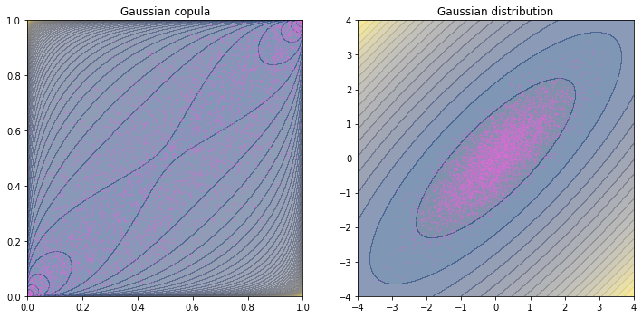
This plot shows that even the copula is a distribution function, it is a distorted one (support is different and the shape is different, too). And in the scatter plot, dots are concentrated at the two opposite corners (i.e., where the p.d.f. peaks) in copula while the they are concentrated at the center in the distribution.
Note that the theme above is on sampling a Gaussian copula in the \(u\)-domain. We are not obligated to convert the random variables in \(u\)-domain to \(x\)-domain using Gaussian marginals as in the plot above.
Example: t coupla
For reference, the \(p\)-dimensional multivariate t distribution with \(\nu\) degrees of freedom has p.d.f.
\[f(\mathbf{x}) = \frac{\Gamma[(\nu+p)/2]}{\Gamma(\nu/2)(\nu\pi)^{p/2}\lvert\boldsymbol{\Sigma}\rvert^{1/2}} \left[ 1+ \frac{1}{\nu} (\mathbf{x}-\boldsymbol{\mu})^\top \boldsymbol{\Sigma}^{-1} (\mathbf{x}-\boldsymbol{\mu}) \right]^{-(\nu+p)/2}\]where \(\boldsymbol{\mu}\) and \(\boldsymbol{\Sigma}\) are the location and shape matrix of the t distribution. In case of standard univariate t, it simplifies into
\[\frac{\Gamma(\frac{\nu+1}{2})}{\Gamma(\frac{\nu}{2})\sqrt{\nu\pi}} \left[ 1+ \frac{x^2}{\nu} \right]^{-(\nu+1)/2}\]The case of t copula:
\[C(\mathbf{u}) = \mathbf{t}_{\nu,P}(t^{-1}_\nu(u_1),\cdots,t^{-1}_\nu(u_d))\]which \(\mathbf{t}_{\nu,P}(\cdot)\) is the multivariate t distribution with \(\nu\) degrees of freedom and correlation matrix \(P\). If \(\mathbf{Z}\) is a standard multivariate Gaussian with correlation \(P\), then with \(\xi \sim \chi^2_{\nu}\) (\(\xi\) is drawn from the \(\chi^2\) distribution with \(\nu\) degrees of freedom),
\[\mathbf{X} = \frac{\mathbf{Z}}{\sqrt{\xi/\nu}}\]follows the \(\mathbf{t(\nu,\mathbf{0},P)}\) distribution.
For the density function, we simply differentiate the copula with the inverse function formula \(\frac{d}{dx} f^{-1}(x) = \frac{1}{f'(f^{-1}(a))}\) and get
\[c(\mathbf{u}) = \frac{\mathbf{t}_{\nu,P}'(t_\nu^{-1}(u_1),\cdots,t_\nu^{-1}(u_d))}{t'_\nu(x_1)\cdots t'_\nu(x_d)}\]Hence we can make use of Gaussian random number generator to sample t copula:
import numpy as np
import scipy as sp
import scipy.stats
import matplotlib.pyplot as plt

# Pearson's correlation and the correlation matrix
# Covariance matrix is just scaling of the correlation matrix
rho = 0.8
corr = np.array([[1, rho],
                 [rho, 1]])
# degrees of freedom
nu = 3

# chi-square random variable
xi = sp.stats.chi2.rvs(nu, random_state=24)
# multivariate Gaussian random numbers
x = sp.stats.multivariate_normal(mean=[0, 0], cov=corr).rvs(5000, random_state=42)
# convert to t distribution
t = x * np.sqrt(nu/xi)
if Fale:
    # In v d.o.f., shape S and covariance matrix C are related with
    #      C = v/(v-2) S
    t = sp.stats.multivariate_t([0,0], corr, df=nu).rvs(5000)
# transform by t CDF
u = sp.stats.t(nu).cdf(t)

# Create pdf contour
axrange = np.linspace(0,1,1000)[1:-1]  # avoid div-by-zero
xv, yv = np.meshgrid(axrange, axrange, indexing='ij') # u,v (CDF) domain
xv2, yv2 = sp.stats.t(nu).ppf(xv), sp.stats.t(nu).ppf(yv) # x,y (PPF) domain
zv = sp.stats.multivariate_t([0,0], corr, df=nu).pdf(np.dstack((xv2, yv2)))
zv /= sp.stats.t(nu).pdf(xv2) * sp.stats.t(nu).pdf(yv2)

# Plot copula
fig = plt.figure(figsize=(12,6))
ax = fig.add_subplot(121)
ax.set_aspect('equal')
ax.set_xlim([0,1])
ax.set_ylim([0,1])
ax.contourf(xv, yv, -np.log(zv), levels=40, alpha=0.5, cmap="cividis")
ax.scatter(u[:,0], u[:,1], c="orchid", s=1.5, alpha=0.3)
ax.set_title("t coupla")

# Contour plot of the t distribution
axrange = np.linspace(-4,4,1000)
xv, yv = np.meshgrid(axrange, axrange, indexing='ij')
zv2 = sp.stats.multivariate_t([0,0], corr, df=nu).pdf(np.dstack((xv, yv)))

# Plot distribution
ax = fig.add_subplot(122)
ax.set_aspect('equal')
ax.set_xlim([-4,4])
ax.set_ylim([-4,4])
ax.contourf(xv, yv, -np.log(zv2), levels=25, alpha=0.5, cmap="cividis")
ax.scatter(t[:,0], t[:,1], c="orchid", s=1.5, alpha=0.3)
ax.set_title("t distribution")
plt.show()
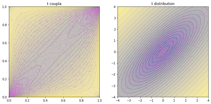
We can see in this plots that t distribution is heavytailed. The copula is more concentrated at the two corners than Gaussian. The distribution is also have denser contours and more spread-out scatters.
Example: Clayton coupla
For bivariate Clayton copula, we can use the conditional distribution approach. With parameter \(\theta\in[-1,\infty)\setminus\{0\}\),
\[C(u_1,u_2) = (u_1^{-\theta} + u_2^{-\theta} - 1)^{-1/\theta}\]The conditional distribution of \(U_2\) given \(U_1=u_1\) is
\[\begin{aligned} C_{u_1}(u_2) &= \Pr[U_2\le u_2\mid U_1=u_1] \\ & = \frac{\partial C(u_1,u_2)}{\partial u_1} \\ &= \frac{-1}{\theta}(u_1^{-\theta} + u_2^{-\theta} - 1)^{-\frac{1+\theta}{\theta}} \cdot -\theta u_1^{-\theta-1} \\ &= (u_1^{-\theta} + u_2^{-\theta} - 1)^{-\frac{1+\theta}{\theta}} \cdot u_1^{-\theta-1} \end{aligned}\]and the inverse is:
\[\begin{aligned} t &= (u_1^{-\theta} + u_2^{-\theta} - 1)^{-\frac{1+\theta}{\theta}} \cdot u_1^{-\theta-1} \\ (u_1^{\theta+1}t)^{-\frac{\theta}{1+\theta}} &= u_1^{-\theta} + u_2^{-\theta} - 1 \\ (u_1^{\theta+1}t)^{-\frac{\theta}{1+\theta}} - u_1^{-\theta} + 1 &= u_2^{-\theta} \\ \big((u_1^{\theta+1}t)^{-\frac{\theta}{1+\theta}} - u_1^{-\theta} + 1\big)^{-1/\theta} &= u_2 \\ \therefore\quad C_{u_1}^{-1}(t) &= \big((u_1^{\theta+1}t)^{-\frac{\theta}{1+\theta}} - u_1^{-\theta} + 1\big)^{-1/\theta} \\ &= \big(u_1^{-\theta}t^{-\frac{\theta}{1+\theta}} - u_1^{-\theta} + 1\big)^{-1/\theta} \\ &= \big(u_1^{-\theta}(t^{-\frac{\theta}{1+\theta}} - 1) + 1\big)^{-1/\theta} \end{aligned}\]and using the method from Nelsen (2006), aka the conditional distribution approach, we can draw \(u_1,t\sim\text{Uniform}(0,1)\) and compute \(u_2 = C_{u_1}^{-1}(t)\), then \((u_1,u_2)\) is a sample from copula \(C\).
import numpy as np
import scipy as sp
import scipy.stats
import matplotlib.pyplot as plt

# Clayton parameter
theta = 1.5  # try -0.98, -0.7, -0.3, -0.1, 0.1, 1, 5, 15, 100
# Uniform random numbers
u1 = np.random.rand(5000)
t = np.random.rand(5000)
# Compute u2 using inverse distribution
u2 = (u1**(-theta) * (t**(-theta/(1+theta)) - 1) + 1)**(-1/theta)

# Contour plot of the copula
kernel = sp.stats.gaussian_kde(np.vstack([u1, u2]))
x = np.linspace(0,1,1000)[1:]  # avoid div-by-zero
xv, yv = np.meshgrid(x, x, indexing='ij')
zv = np.reshape(kernel(np.vstack([xv.ravel(), yv.ravel()])).T, xv.shape)

# Plot
fig = plt.figure(figsize=(12,6))
ax = fig.add_subplot(121)
ax.set_aspect('equal')
ax.set_xlim([0,1])
ax.set_ylim([0,1])
ax.scatter(u1, u2, c="orchid", s=1.5, alpha=0.3)
ax.set_title("Clayton copula")

ax = fig.add_subplot(122)
ax.set_aspect('equal')
ax.set_xlim([0,1])
ax.set_ylim([0,1])
ax.contourf(xv, yv, -zv, levels=50, cmap="cividis")
ax.set_title("Clayton copula KDE")
plt.show()
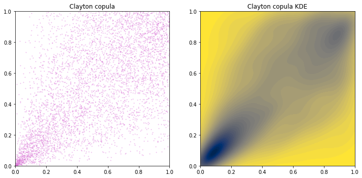
Note that we don’t have a Clayton distribution. And I don’t know how to get a close-form density function of Clayton copula, hence KDE is used instead.
From the copula plot, we see that Clayton copula is asymmetric in the sense that density around \(u_1=u_2=0\) is much higher than that around \(u_1=u_2=1\). Hence \(u_1\) and \(u_2\) are stronger correlated at left tail.
Example: Gumbel coupla
The bivariate Gumbel copula with parameter \(\theta\in[1,\theta)\) is
\[C(u_1,u_2) = \exp\Big(-\big((-\ln u_1)^\theta + (-\ln u_2)^\theta\big)^{1/\theta}\Big)\]We do not have a close form inverse function for the conditional distribution \(C_{u_1}(u_2) = \Pr[U_2\le u_2\mid U_1=u_1]\).
Gumbel copula is an Archimedean copula, which means \(C(u,v)=C(v,u)\) and can be expressed in the form of
\[C(u,v) = \phi^{-1}\big(\phi(u)+\phi(v))\]which in case of Gumbel, \(\phi(v)=(-\ln v)^\theta\) (and hence \(\phi^{-1}(t) = \exp(-t^{1/\theta})\) as the inverse).
Sampling an Archimedean copula can use the following algorithm:
- Generate \(v_1, v_2\sim\text{Uniform}(0,1)\)
- Set \(K_C(t) = t - \dfrac{\phi(t)}{\phi'(t)}\) and \(w=K_C^{-1}(v_2)\)
- Set \(u_1=\phi^{-1}\big(v_1\phi(w)\big)\) and \(u_2=\phi^{-1}\big((1-v_1)\phi(w)\big)\)
In case of Gumbel, \(\phi'(v) = \dfrac{-\theta}{v}(-\ln v)^{\theta-1}\) and
\[\begin{aligned} K_C(v) &= v - \frac{(-\ln v)^{\theta}}{\frac{-\theta}{v}(-\ln v)^{\theta-1}} \\ &= v + \frac{v}{\theta}(-\ln v) = v - \frac{v}{\theta}\ln v \\ &= v\Big(1-\frac{\ln v}{\theta}\Big) \end{aligned}\]The parameter \(\theta\) is related to the Kendall’s rank correlation by \(\tau = 1-1/\theta\).
For reference, a standard Gumbel distribution has p.d.f. and c.d.f.
\[\begin{aligned} f(x) &= \exp(-x-e^{-x}) \\ F(x) &= \exp(-e^{-x}) \end{aligned}\]import numpy as np
import scipy as sp
import scipy.stats
import matplotlib.pyplot as plt
# K_C(v) function
def KC(v,theta):
return v * (1-np.log(v, where=v!=0)/theta)
# phi function and inverse
def phi(v,theta):
return np.power(-np.log(v), theta)
def phiinv(t, theta):
return np.exp(-np.power(t, 1/theta))
# Gumbel parameter
theta = 2 # Try 1.1, 1.5, 2, 4, 8, 50
# Define function for interpolation
# K_C(v) is monotonically increasing thus np.interp(x,xp,fp) works
x = np.linspace(0,1,10000)
y = KC(x,theta)
# Uniform random numbers
v = np.random.rand(5000,2)
# Compute w from inverse of KC
w = np.interp(v[:,1], y, x)
# Compute u_1 and u_2
u1 = phiinv(v[:,0] * phi(w,theta), theta)
u2 = phiinv((1-v[:,0]) * phi(w,theta), theta)
# Contour plot of the copula
kernel = sp.stats.gaussian_kde(np.vstack([u1, u2]))
axrange = np.linspace(0,1,1000)[1:-1] # avoid div-by-zero
xv, yv = np.meshgrid(axrange, axrange, indexing='ij')
zv = np.reshape(kernel(np.vstack([xv.ravel(), yv.ravel()])).T, xv.shape)
# Plot
fig = plt.figure(figsize=(12,6))
ax = fig.add_subplot(121)
ax.set_aspect('equal')
ax.set_xlim([0,1])
ax.set_ylim([0,1])
ax.contourf(xv, yv, -zv, levels=50, cmap="cividis")
ax.scatter(u1, u2, c="orchid", s=1.5, alpha=0.3)
ax.set_title("Gumbel coupla")
# Distribution plot derived from copula
x = sp.stats.gumbel_r.ppf(u1)
y = sp.stats.gumbel_r.ppf(u2)
# Contour plot of the distribution
kernel = sp.stats.gaussian_kde(np.vstack([x, y]))
axrange = np.linspace(-2,6,1000)[1:-1] # avoid div-by-zero
xv, yv = np.meshgrid(axrange, axrange, indexing='ij')
zv = np.reshape(kernel(np.vstack([xv.ravel(), yv.ravel()])).T, xv.shape)
# Plot distribution
ax = fig.add_subplot(122)
ax.set_aspect('equal')
ax.set_xlim([-2,6])
ax.set_ylim([-2,6])
ax.contourf(xv, yv, -zv, levels=50, cmap="cividis")
ax.scatter(x, y, c="orchid", s=1.5, alpha=0.3)
ax.set_title("Gumbel distribution")
plt.show()
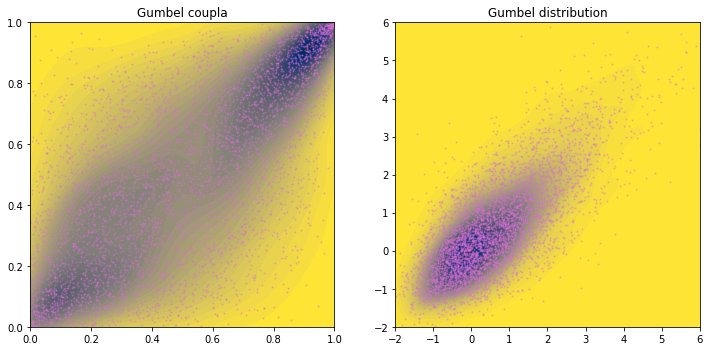
The Gumbel distribution is a skewed distribution (long tail to the right). Hence we see a pointy tail toward positive \(x\) and \(y\) corner. From the copula plot, we conclude that \(x\) and \(y\) are stronger correlated at the right tail.
Correlation and marginal distribution
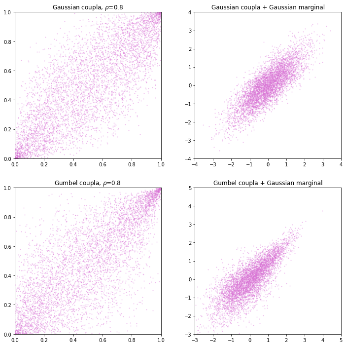
Knowing the linear correlation and the marginal distribution of two random variables does not uniquely identifies their joint distribution. For example, generate a Gaussian and Gumbel copula with same linear correlation, then transform the sample using Gaussian distribution. The result is to have the distribution in oval shape (Gaussian copula) and teardrop shape (Gumbel copula).
In Gaussian, Kendall’s \(\tau\) and Pearson’s \(\rho\) are related by
\[\tau = \frac{2}{\pi}\sin^{-1}\rho\]which we can make the following:
import numpy as np
import scipy as sp
import scipy.stats
import matplotlib.pyplot as plt
from matplotlib import cm


# Pearson's correlation and the correlation matrix
rho = 0.8
corr = np.array([[1, rho],
                 [rho, 1]])
# Kendall's tau
tau = 2/np.pi * np.arcsin(rho)
# Gumbel distribution parameter
theta = 1/(1-tau)


# Sample from Gaussian copula
# using scipy to generate multivariate normal rng
x_gau = sp.stats.multivariate_normal(mean=[0, 0], cov=corr).rvs(5000)
u_gau = sp.stats.norm.cdf(x_gau)


# Interpolation curve for Gumbel copula
# K_C(v) function
def KC(v,theta):
    return v * (1-np.log(v, where=v!=0)/theta)
# phi function and inverse
def phi(v,theta):
    return np.power(-np.log(v), theta)
def phiinv(t, theta):
    return np.exp(-np.power(t, 1/theta))
# Generate the curve
x = np.linspace(0,1,10000)
y = KC(x,theta)

# Sample from Gumbel copula
v = np.random.rand(5000,2)
w = np.interp(v[:,1], y, x)
# Compute u_1 and u_2
u_gum1 = phiinv(v[:,0] * phi(w,theta), theta)
u_gum2 = phiinv((1-v[:,0]) * phi(w,theta), theta)

# Transform from Gaussian marginal
x_gum1 = sp.stats.norm.ppf(u_gum1)
x_gum2 = sp.stats.norm.ppf(u_gum2)

# Plot: Gaussian
fig = plt.figure(figsize=(12,12))
ax = fig.add_subplot(221)
ax.set_aspect('equal')
ax.set_xlim([0,1])
ax.set_ylim([0,1])
ax.scatter(u_gau[:,0], u_gau[:,1], c="orchid", s=1.5, alpha=0.3)
ax.set_title(r"Gaussian coupla, $\rho$=0.8")

ax = fig.add_subplot(222)
ax.set_aspect('equal')
ax.set_xlim([-4,4])
ax.set_ylim([-4,4])
ax.scatter(x_gau[:,0], x_gau[:,1], c="orchid", s=1.5, alpha=0.3)
ax.set_title("Gaussian coupla + Gaussian marginal")

# Plot: Gumbel
ax = fig.add_subplot(223)
ax.set_aspect('equal')
ax.set_xlim([0,1])
ax.set_ylim([0,1])
ax.scatter(u_gum1, u_gum2, c="orchid", s=1.5, alpha=0.3)
ax.set_title(r"Gumbel coupla, $\rho$=0.8")

ax = fig.add_subplot(224)
ax.set_aspect('equal')
ax.set_xlim([-3,5])
ax.set_ylim([-3,5])
ax.scatter(x_gum1, x_gum2, c="orchid", s=1.5, alpha=0.3)
ax.set_title("Gumbel coupla + Gaussian marginal")

plt.show()
Optionally, we can check the correlation matrix to verify that the linear correlation (Pearson’s \(\rho\)) of the two dataset matches:
print(np.corrcoef(x_gau[:,0], x_gau[:,1]))
print(np.corrcoef(x_gum1, x_gum2))
Pearson’s \(\rho\) depends on the marginal distribution of each random variable. Hence we cannot tell the Pearson correlation from copula functions. However, rank correlation can be derived from copula functions.
The Kendall’s \(\tau\) is defined as
\[\begin{aligned} \tau(X,Y) &= \mathbb{E}[\textrm{sign}((X-X')(Y-Y'))] \\ &= \mathbb{P}[(X-X')(Y-Y')>0] - \mathbb{P}[(X-X')(Y-Y')<0] \end{aligned}\]for \((X,Y)\) and \((X',Y')\) are independent pairs drawn from the same distribution. If the marginals are continuous, we can express the Kendall’s \(\tau\) in copula:
\[\tau(X,Y) = 4 \int_0^1 \int_0^1 C(x,y)\; dC(x,y) - 1\]There is also Spearman’s \(\rho\), which is also a rank correlation and defined as
\[\rho_s(X,Y) = \rho(F_X(X), F_Y(Y))\]i.e., the Pearson’s correlation in \([0,1]\) domain transformed by c.d.f. In fact, it is natural to use Spearman’s \(\rho\) with copula because as long as the marginals are continuous,
\[\rho_s(X,Y) = 12 \int_0^1\int_0^1 (C(x,y)-xy)\;dx\;dy\]and in case of Gaussian copula,
\[\rho_s = \frac{6}{\pi}\sin^{-1}\frac{\rho}{2} \approx \rho\]Rank correlations are consistent under monotonic transformations. Hence it is a perfect fit to copula functions.
Dependence of copula and the correlation coefficients
Fréchet-Hoeffding Bounds says: All copula \(C(\mathbf{u})=C(u_1,\cdots,u_d)\) satisfies
\[\max\Big\{1-d+\sum_{i=1}^d u_i, 0\Big\} \le C(\mathbf{u}) \le \min\{u_1,\cdots,u_d\}\]Comonotonic copula is the one at the upperbound:
\[C(\mathbf{u}) = \min\{u_1,\cdots,u_d\}\]Countermonotonic copula (exists only for \(d=2\)) is the one at the lowerbound:
\[W(u_1,u_2) = \max\{u_1+u_2-1, 0\}\]Independence copula is the one:
\[C(\mathbf{u}) = \prod_{i=1}^d u_i\]Comonotonic copula is those with extreme positive dependence (Spearman’s \(\rho\) and Kendall’s \(\tau\) are 1). Countermonotonic copula is the case of perfect negative dependence (Spearman’s \(\rho\) and Kendall’s \(\tau\) are \(-1\)).
References
- Martin Haugh (2016) An Introduction to Copulas, IEOR E4602 Quantitative Risk Management Lecture Notes
- Copula methods: Modelling correlation between risks, and its slides
- Procedure to Generate Uniform Random Variates from Each Copula
- Nelsen, R. B. (2006) An Introduction to Copulas (2nd ed.), Springer-Verlag, New York